
5 Genomic Variation and Polygenic Scores
Reading Objectives
By the end of this chapter, you should be able to:
- Trace how a biological specimen becomes genomic data and distinguish genotyping-array, whole-genome sequencing, and imputed genotype resources.
- Explain how a defined phenotype and discovery sample produce GWAS evidence, and interpret a Manhattan plot without making unsupported causal claims.
- Explain how effect alleles, allele dosages, and GWAS weights are combined to construct a polygenic score.
- Distinguish discovery data from target data, score construction from evaluation, and group-level associations from individual predictions.
- Interpret standardized scores, percentiles, quantile groups, outcome gradients, and common measures of prediction performance.
- Explain why PGS performance changes across populations and contexts, and distinguish genetic ancestry from race, ethnicity, and social experience.
- Identify gene-environment interaction, gene-environment correlation, and governance safeguards relevant to responsible genomic research.
Key Terms
Genome · chromosome · genomic locus · genetic variant · single-nucleotide polymorphism (SNP) · allele · genotype · effect allele · allele dosage · genotyping array · whole-genome sequencing · imputation · genome-wide association study (GWAS) · discovery sample · genetic principal components · genome-wide significance threshold · replication sample · Manhattan plot · polygenic score (PGS) · polygenic risk score (PRS) · target sample · standardized score (z-score) · quantile group · genetic ancestry · gene-environment interaction (G×E) · gene-environment correlation (rGE) · genomic-data governance
1. Introduction
How can a tube of saliva become a number that researchers use to study someone’s likelihood of substance use?
The journey is surprisingly long. DNA must be extracted and measured, genetic differences must be represented as data, and those data must be linked to carefully defined outcomes. Researchers can then test millions of genetic variants in a genome-wide association study, or combine many small associations into a polygenic score. By the end of that process, a participant may have a single numeric value representing part of the genetic variation statistically associated with a measured outcome.
But what does that number actually mean?
It does not identify an “addiction gene,” determine whether someone will develop a substance use disorder, or separate people into biologically distinct racial groups. Its meaning depends on what phenotype was measured, who was included in the study, how the genomic data were processed, which statistical model was used, and the social and developmental conditions in which the association was observed.
Chapter 4 introduced behavioral genetics by asking why relatives and twins resemble one another. This chapter moves from patterns of inheritance to measured DNA variation. We follow the genomic data journey from a biological specimen to genome-wide association studies (GWAS), then from GWAS results to polygenic scores (PGS). Along the way, we examine how scores are constructed and evaluated, why their performance changes across populations and contexts, and why genomic associations cannot be interpreted apart from measurement, environment, and study design.
The chapter ends with a real case of restricted child genomic data being used to make unsupported claims about race and intelligence. That case brings the chapter’s central lesson into focus: genomic data can be powerful evidence, but the meaning of that evidence depends on how the data were produced, analyzed, interpreted, and governed.
2. From a biospecimen to genomic data
Chapter 4 investigated inherited variation without measuring specific DNA differences. This section follows how a biological specimen becomes genomic data, which researchers use for genome-wide association studies (GWAS) and polygenic scores (PGS).
2.1 The minimum genomic vocabulary
DNA and phenotype were introduced in Chapter 4. Figure 5.1 introduces the additional vocabulary needed to understand how researchers represent genetic variation in GWAS and polygenic scores. Read the figure as a sequence of increasingly focused views: from the genome, to a chromosome, to a particular locus, and finally to the alleles and genotypes recorded at one SNP.
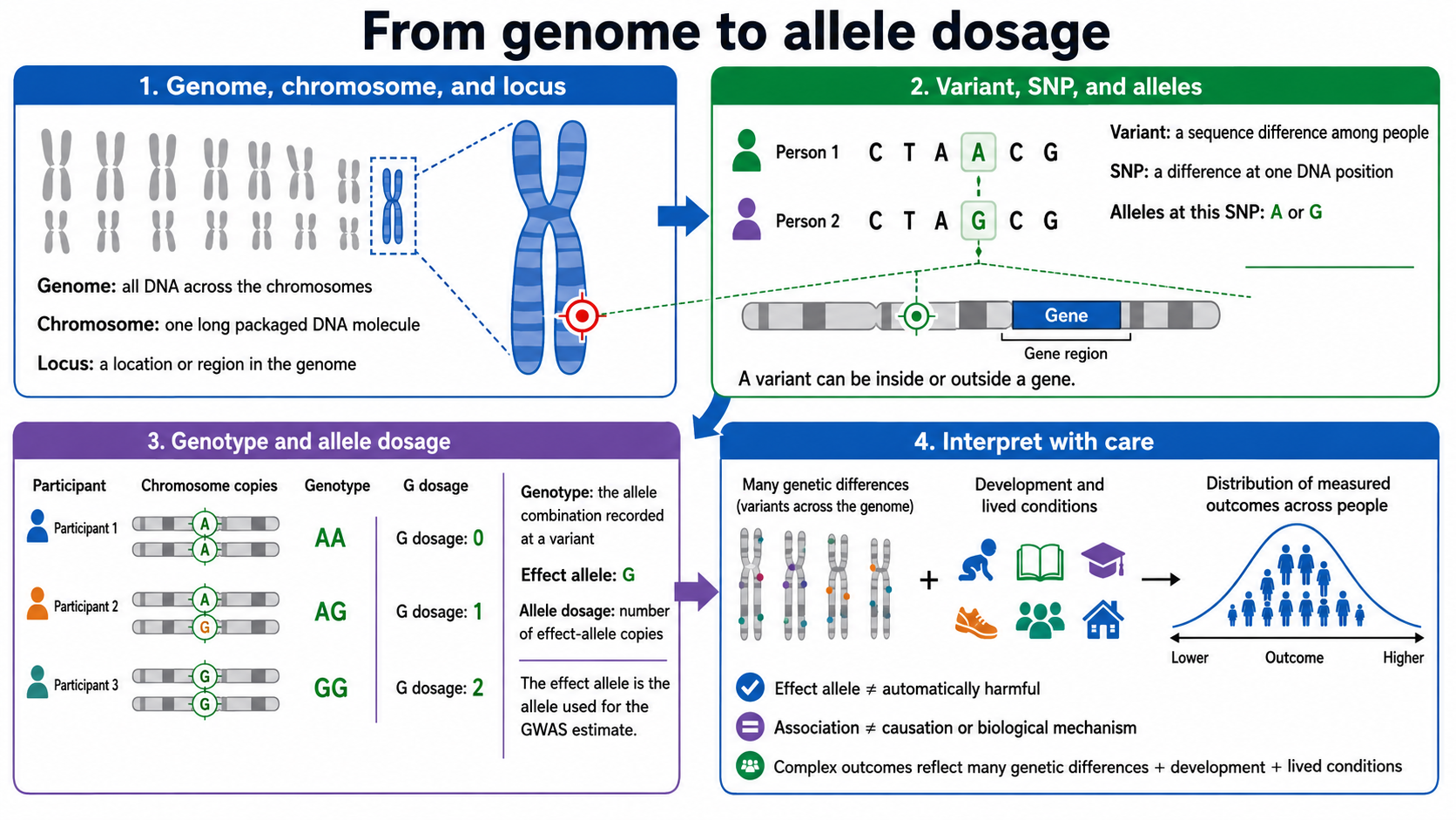
The designation effect allele identifies which allele a reported GWAS estimate describes. It does not mean that the allele is harmful or that it causes the measured outcome. The same allele can also be associated with higher values in one analysis and lower values in another, depending on how the outcome and estimate are defined.
A variant may occur inside or outside a gene. Even when a variant is located within or near a gene, its location alone does not establish that the gene explains an association. Addiction-related outcomes are related to thousands of genetic differences together with development and lived conditions.
2.2 The physical and operational journey
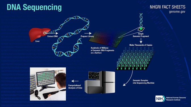
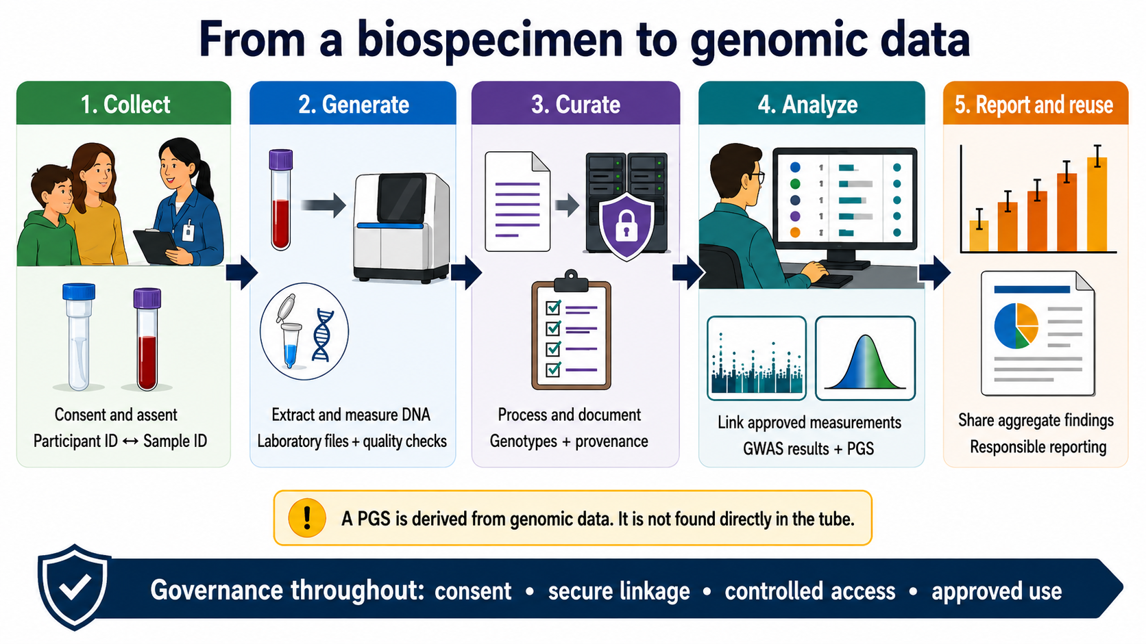
Genomic data collection begins after a youth and caregiver complete assent and consent procedures for sample collection and genomic sequencing (assent is the youth’s voluntary, age‑appropriate agreement to participate, while consent is the caregiver’s legally valid authorization). Staff then collect saliva or blood using a documented protocol. The original ABCD protocol described site-level ethics approval, participant consent and assent, baseline saliva collection, repository shipment, storage, DNA isolation, and blood collection for part of the twin sample (Uban et al., 2018).
The specimen receives a controlled sample identifier linked to the participant record. The two identifiers serve different purposes: a participant identifier refers to a person, while a sample identifier refers to a particular tube, collection, or extracted portion. The specimen is stored, transported, and processed under documented conditions. Laboratory staff isolate DNA, assess its quantity and quality, and use a genotyping array or sequencing instrument to generate laboratory files. Quality checks may identify contamination, low-quality results, unexpected relatedness, or disagreement between records and genetic data. Files then move through secure systems for additional processing, documentation, and linkage to approved outcome measurements.
This sequence explains why laboratory output is not immediately an analysis-ready dataset. Each stage can change what is available for analysis. Good provenance records the specimen source, data release, laboratory platform, processing pipeline, reference genome, quality-control decisions, and software or file version.
2.3 Genomic resources in ABCD
ABCD provides several related genomic resources. Genotyping-array data record selected variants measured using probes on an array. Whole-genome sequencing data are produced by reading DNA across the genome and aligning the reads to a reference sequence. Both resources require quality review.
Imputed genotype data add statistically estimated genotypes at variants that were not directly measured on the array. The estimates use observed genotypes and patterns in a reference resource. An imputed allele dosage can therefore be a value between 0 and 2, reflecting uncertainty, rather than a directly observed count. Imputation expands genomic coverage, but it does not mean that every DNA position was directly observed.
ABCD also provides sample-level and variant-level quality information, estimates of genetic relatedness, and principal components, which are numeric variables summarizing major patterns of genomic similarity among participants. Relatedness measures help identify family relationships and account for nonindependence. Principal components help researchers address population structure that could otherwise create misleading associations.
ABCD Release 7.0 note. Release 7.0 includes curated Smokescreen array data for 11,670 participants at about 515,000 variants, imputed array data for the same participants at about 260 million variants, and 30x Illumina whole-genome sequencing for 8,710 participants at about 169 million variants. Counts depend on the resource and quality-control rules and should not be treated as permanent study characteristics. Record the release, retrieval date, platform, and analytic sample whenever reporting results. (ABCD genetics documentation; Release 7.0 notes)
2.4 One resource, several data structures
A conceptual genotype matrix has participants in rows and variants in columns, with each cell containing a genotype or dosage. Real genomic resources are too large and specialized to remain in one ordinary DataFrame. VCF files can store variant and genotype information, while PLINK files provide another specialized representation used in genetic analysis. We do not work with these files in this course; instead, we use synthetic versions of derived data.
Later steps create different structures for different purposes. GWAS summary statistics usually contain one row per tested variant, along with its effect allele, estimated association, and uncertainty. A PGS scoring file contains the variants, effect alleles, and weights used to construct a score. An analysis-ready participant table may then contain one standardized PGS per participant, together with selected outcomes and contextual variables. The PGS is therefore a derived variable, not raw biological data.
2.5 Governance throughout the journey
Removing names does not eliminate genomic privacy risks. A person’s genomic data can be highly identifying, and they are relational because they can also reveal information about biological relatives. Data collected from youth may later support research questions that participants and families did not anticipate at enrollment. Linking specimens, participant records, genomic files, and outcomes therefore requires controlled identifiers, approved systems, and continuing oversight.
For these reasons, the Data Use Certificate that we covered in Module 1 illustrated that controlled access to ABCD data is more than a password. Genomic data requests to ABCD consider the investigator and institution, the proposed purpose, the computing environment, the specific data requested, plans for storage and sharing, reporting procedures, deletion requirements, and compliance with prior agreements. We explore these issues more at the end of this chapter.
3. From a measured outcome to GWAS evidence
Section 2 described how biological specimens become genomic data and how those data are structured. Section 3 asks how researchers test whether genetic variants are associated with measured phenotypes.
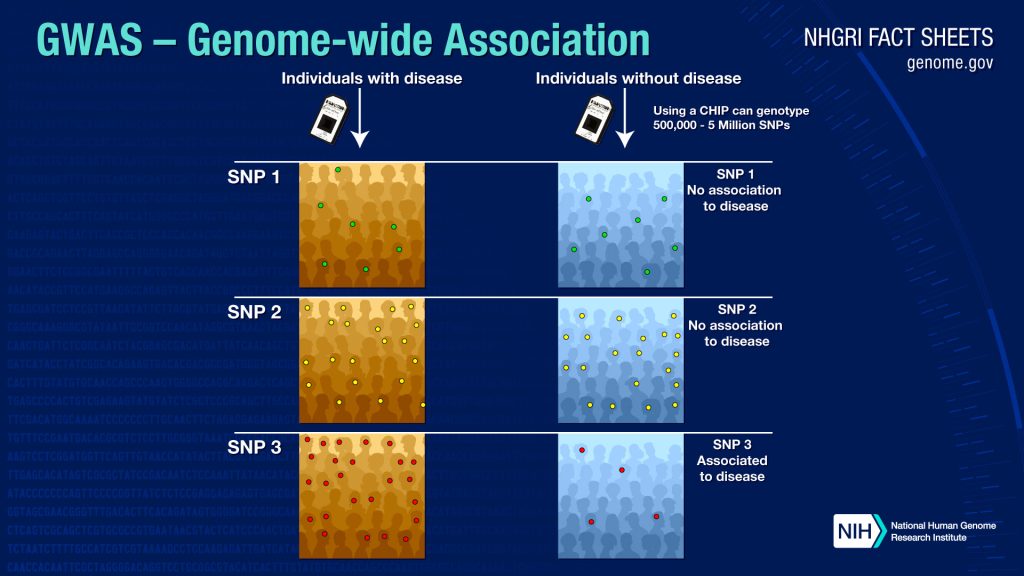
A genome-wide association study (GWAS) examines genetic variants across the genome to determine whether any are associated with a measured outcome. Researchers study many participants and test hundreds of thousands or millions of variants, usually single-nucleotide polymorphisms (SNPs).
The illustration below shows the basic logic using a binary disease outcome. Researchers compare allele frequencies between participants with and without the disease. If an allele is more frequent in one group, that variant may show evidence of association with the measured outcome.
3.1 The measured outcome comes first
Chapters 2 through 4 followed the measurement process:
Construct → instrument or procedure → recorded value → scoring process → analytic variable → interpretation
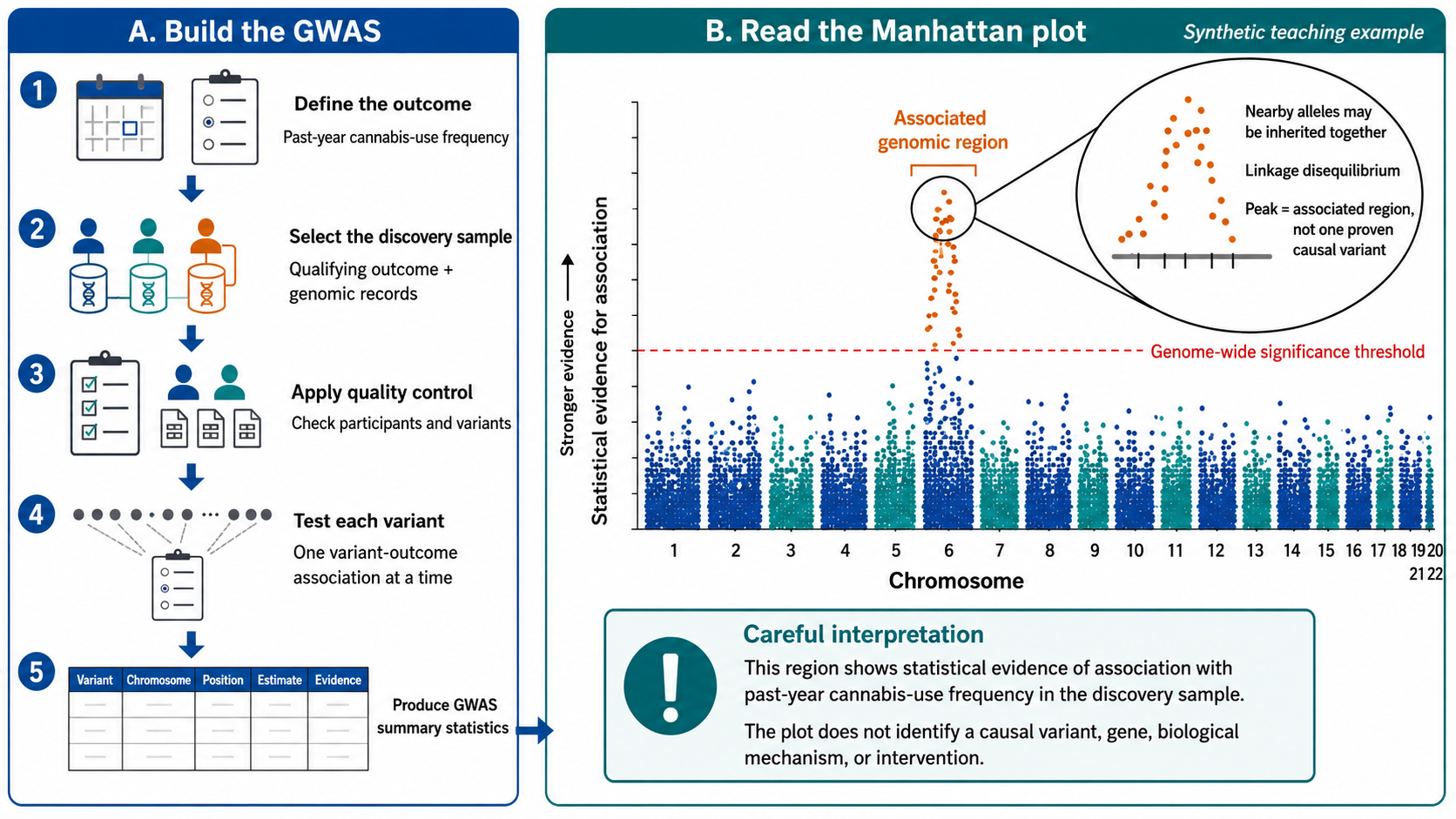
The same sequence applies in a GWAS. Researchers must specify the phenotype, the instrument or procedure used to measure it, and the analytic variable that will represent it. “A GWAS of addiction” is not sufficiently precise.
Returning to Figure 5.3 above, applied to addiction research, what exactly counts as “with” or “without” the outcome? Addiction research may instead examine frequency of use, number of use days, symptom counts, or a broader behavioral score. These measurement decisions made before the genetic analysis determine what the GWAS results mean, as they answer different research questions and may produce different genomic associations.
3.2 The discovery sample and GWAS process
The discovery sample consists of the participants whose genomic and outcome data are used to estimate associations. Researchers define eligibility rules, identify qualifying records, apply quality controls, account for relevant study characteristics and population structure, and test variants across the genome.
In a case-control GWAS, researchers ask whether genotypes differ systematically between participants who meet specified criteria and those who do not. GWAS can also examine continuous measures, such as an externalizing score, or counts, such as reported days of cannabis use. The statistical model must match the outcome.
GWAS summary statistics commonly record each variant, its genomic position and effect allele, its estimated association, uncertainty, and statistical evidence. They summarize results across the discovery sample rather than providing one row per participant.
3.3 Quality control and population structure
Quality checks may identify incomplete records, poorly measured variants, duplicate samples, unexpected biological relationships, differences across laboratory batches or platforms, and low-quality imputed genotypes. These checks can change both the analytic sample and the variants tested.
Researchers must also consider population structure, meaning patterned genomic similarity related to population histories. Without appropriate adjustment, an analysis may detect background population differences rather than the relationship of interest. Genetic principal components summarize some major patterns of genomic similarity and are often included in GWAS models. They do not represent natural divisions of people into genetic groups.
3.4 Testing many variants and seeking replication
A GWAS evaluates hundreds of thousands or millions of variant-outcome associations. Conducting so many tests creates many opportunities for apparently strong results to occur by chance. Researchers therefore use a stringent genome-wide significance threshold as one safeguard.
Crossing the threshold indicates strong statistical evidence under the model. It does not mean that the association is large, clinically useful, causal, or biologically understood. Calculating p-values and multiple-testing corrections is reserved for DSARM 2. Here, the goal is interpreting the threshold.
A replication sample is a separate sample used to examine whether an important association appears again. Replication reduces the possibility that a finding reflects chance or a feature unique to one sample. It strengthens confidence in an association but does not prove a biological mechanism.
3.5 Reading a Manhattan plot
A Manhattan plot displays GWAS results across the genome. The horizontal axis shows genomic position, grouped by chromosome. Each point represents one tested variant. The vertical axis represents the strength of statistical evidence for its association with the measured outcome, so higher points indicate stronger evidence. A horizontal line marks the genome-wide significance threshold.
Several high points may appear together because of linkage disequilibrium, meaning that particular alleles at nearby locations tend to be inherited together. One measured variant may therefore tag another in the same region. A peak usually identifies an associated genomic region, not one proven causal nucleotide. Assigning the peak to the nearest gene is an annotation step, not proof that the gene explains the association. A careful interpretation is: This region shows statistical evidence of association with the measured outcome in the discovery sample.
3.6 Running example and research extension
The synthetic example in Figure 5.4 uses past-year cannabis-use frequency as the measured outcome. Every point represents a test of one variant against that same defined variable in the qualifying discovery sample. Because the data are synthetic, the peak illustrates how to read the plot and does not make a claim about an actual genomic region.
Research extension: Multivariate GWAS
Some studies model several related outcomes together. A 2026 study combined substance-use-disorder and other externalizing GWAS representing more than 2.2 million participants. The researchers examined associations shared across broad externalizing behavior and associations more specific to particular substance-use disorders. Combining outcomes can improve detection of small associations, but it changes what the analysis represents. Large sample size also does not guarantee broad population coverage. The study included only participants classified as having European genetic ancestry, limiting the populations to which its findings can be generalized (Poore et al., 2026).
4. From GWAS associations to a polygenic score
Section 3 ended with GWAS summary statistics. These results contain an estimated association for each tested variant. Researchers can combine estimates across many variants to construct a polygenic score (PGS) for participants in another dataset.
A PGS summarizes selected genetic differences as one numeric variable. It is called polygenic because it combines information from many locations across the genome. The score does not reveal whether an outcome will occur. Its usefulness must be evaluated by examining how strongly it is associated with a measured outcome in appropriate data.
4.1 Preferred terminology
Polygenic score is the general term used in this chapter. A PGS can be constructed for a continuous measure, such as height, cannabis-use frequency, or an externalizing score, as well as for a diagnosis or other binary outcome.
The term polygenic risk score (PRS) is sometimes used when the score is explicitly constructed for a disease or adverse binary outcome. “Risk” is less appropriate when the GWAS outcome is a continuous measure or when higher values are not inherently harmful. Regardless of the name, the score is calculated using the same general weighted-sum logic.
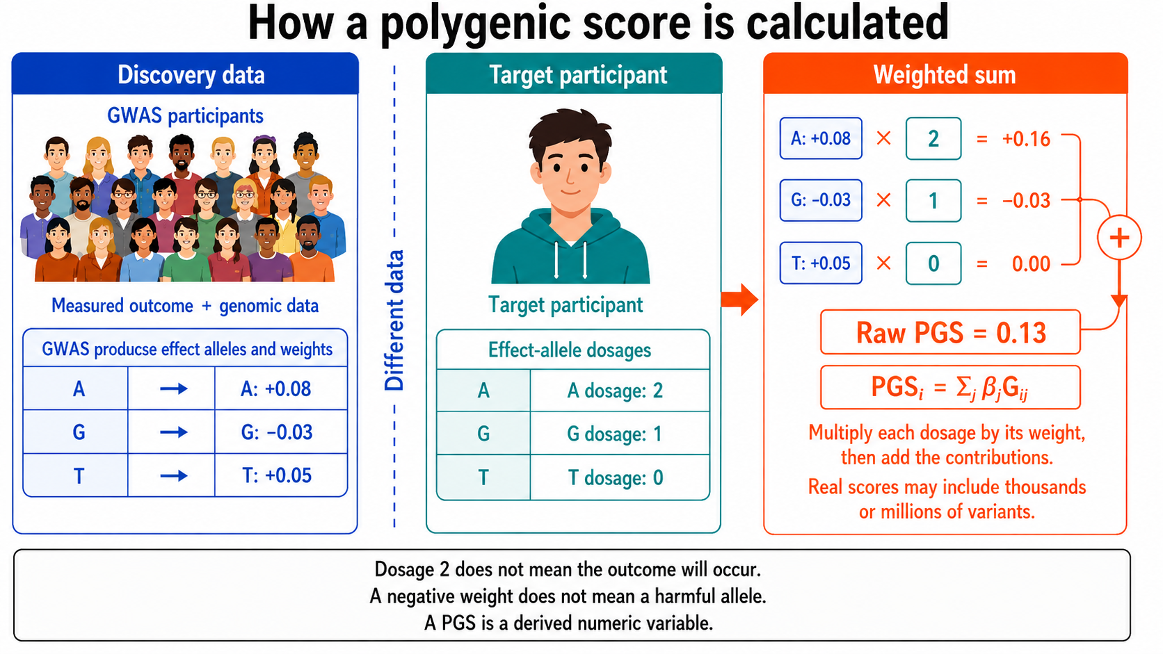
4.2 Discovery data and target data
PGS construction involves two conceptually separate sources of data:
- Discovery data supply the GWAS estimates used as scoring weights.
- Target data contain the participants for whom the score is calculated and evaluated.
Suppose a GWAS tests past-year cannabis-use frequency in a large discovery sample. For each variant, the resulting summary statistics identify an effect allele and estimate how dosage of that allele is associated with the measured outcome. Those estimates can then be applied to qualifying genotype data from target participants.
The target data must contain compatible genomic positions, allele definitions, and genotype or dosage information. Researchers also need relevant quality-control records and a documented outcome against which the score can be evaluated. A score cannot be interpreted responsibly if researchers do not know which GWAS supplied its weights or how the target genotypes were processed.
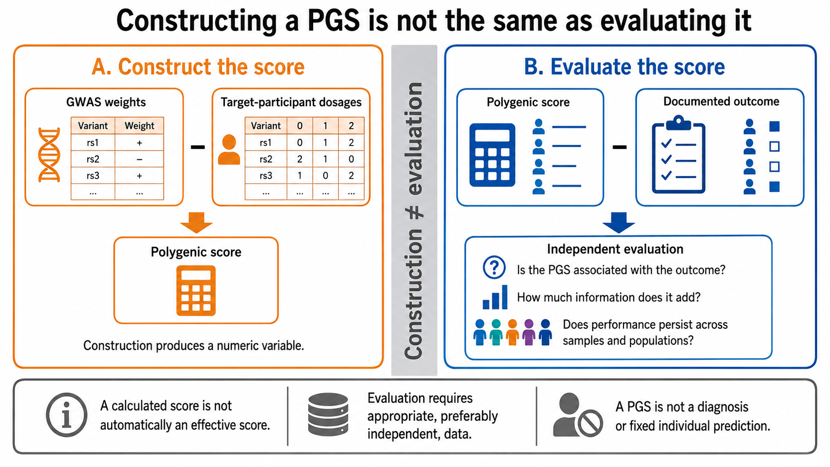
Discovery and evaluation participants should remain appropriately separate. If the same participants are casually used both to estimate variant weights and to evaluate the resulting score, apparent performance may be inflated because the score is partly being assessed against the data that produced it. Researchers can use independent samples or carefully designed validation procedures to reduce this problem.
4.3 Effect alleles, dosages, and weights
For every included variant, the scoring procedure needs a variant identifier, an effect allele, a weight, and the target participant’s effect-allele dosage. The alleles must be aligned correctly so that the weight and dosage refer to the same allele.
Consider a fictional score containing three variants:
| Variant | Effect allele | Weight | Participant dosage | Weighted contribution |
|---|---|---|---|---|
| Variant 1 | A | +0.08 | 2 | +0.16 |
| Variant 2 | G | −0.03 | 1 | −0.03 |
| Variant 3 | T | +0.05 | 0 |
For each row, the dosage is multiplied by the weight. The contributions are then added:
In this expression, PGSi is the score for participant i. The symbol βj represents the weight assigned to variant j, and Gij represents participant i’s dosage of the effect allele at that variant. The summation symbol means to repeat the multiplication across the included variants and add the results.
For the participant in the table, the raw score is:
(0.08 × 2) + (−0.03 × 1) + (0.05 × 0) = 0.13
The important idea is the weighted sum, not memorizing the notation. A dosage of 2 means that the participant has two copies of the designated effect allele. It does not mean that the outcome will occur. Similarly, a negative weight indicates the direction of an estimated association under a particular outcome definition and coding scheme. It does not identify a harmful, protective, or defective allele.
Real scores may combine hundreds, thousands, or millions of variants. Each weight may be very small, but the combined score can still show an aggregate association with the outcome.
4.4 Variant selection and correlation
Researchers must also decide which variants and weights to include. Nearby variants can carry overlapping information because of linkage disequilibrium, introduced in Section 3. A scoring method must therefore address correlation among variants.
Some methods select variants that are relatively independent of one another. Other methods model many correlated variants jointly. Modern approaches differ in their assumptions, required reference data, and treatment of uncertainty. No single simplified procedure represents every valid PGS method, and selecting variants through one thresholding procedure is not the definition of PGS construction (Choi et al., 2020).
4.5 What a PGS represents
A PGS is a derived numeric variable tied to a particular source GWAS and scoring method. Its meaning depends on how the GWAS outcome was defined, who participated in the discovery sample, which variants were included, how weights were estimated, and how the target data were processed.
The score captures only part of the genetic variation statistically associated with the measured outcome. It is not an environmental measure, diagnosis, or fixed prediction of an individual’s future. It also should not be assumed to perform identically across populations or settings.
A PGS is not the same as heritability. Heritability describes the proportion of variation in a measured phenotype attributed to genetic differences under a particular population and model. A PGS is one measured variable constructed from selected variants and weights.
4.6 Provenance requirements
A column name such as cannabis_pgs is not sufficient documentation for a derived variable. Researchers should identify the target outcome, source GWAS, discovery sample, genome build, variant identifiers, effect alleles and weights, scoring method, software version, quality-control rules, and target-sample inclusion criteria. Documentation should also specify any standardization reference, the evaluation sample, and the performance measures reported. These documentation requirements are consistent with established reporting standards for PGS construction, validation, and interpretation (Wand et al., 2021).
4.7 Independent evaluation
Calculating a score does not establish that it performs well. Score construction combines weights and allele dosages. Score evaluation examines the relationship between the resulting PGS and a documented outcome.
Evaluation asks whether the PGS is associated with its intended outcome, how large that association is, and whether the score adds information beyond a reasonable baseline model. Researchers should also ask whether performance persists in an independent sample and whether it is similar across relevant populations and settings. PGS performance can differ substantially across populations, partly because discovery GWAS have not represented populations equally (Martin et al., 2019).
5. From scores to distributions and outcome gradients
Section 4 explained how researchers combine GWAS weights and participant allele dosages to construct a polygenic score. Once scores have been calculated for many participants, researchers can examine their distribution and evaluate their association with a measured outcome. This requires careful attention to units, reference samples, group averages, and individual variation.
5.1 Why raw PGS values are difficult to interpret
A raw PGS is the sum of weighted allele dosages. Its numerical scale depends on which variants were included, which alleles were designated as effect alleles, the scale of the weights, the source GWAS, the scoring method, and genomic-processing decisions.
For one score, raw values might range from −0.4 to +0.6. Another might range from −12 to +15. These differences do not mean that the second score captures more genetic variation or predicts its outcome better. The two scores simply use different units. Raw values from different PGS therefore cannot ordinarily be compared directly.
Even within one study, a raw value has little meaning unless its construction and reference distribution are documented.
5.2 Standardized scores
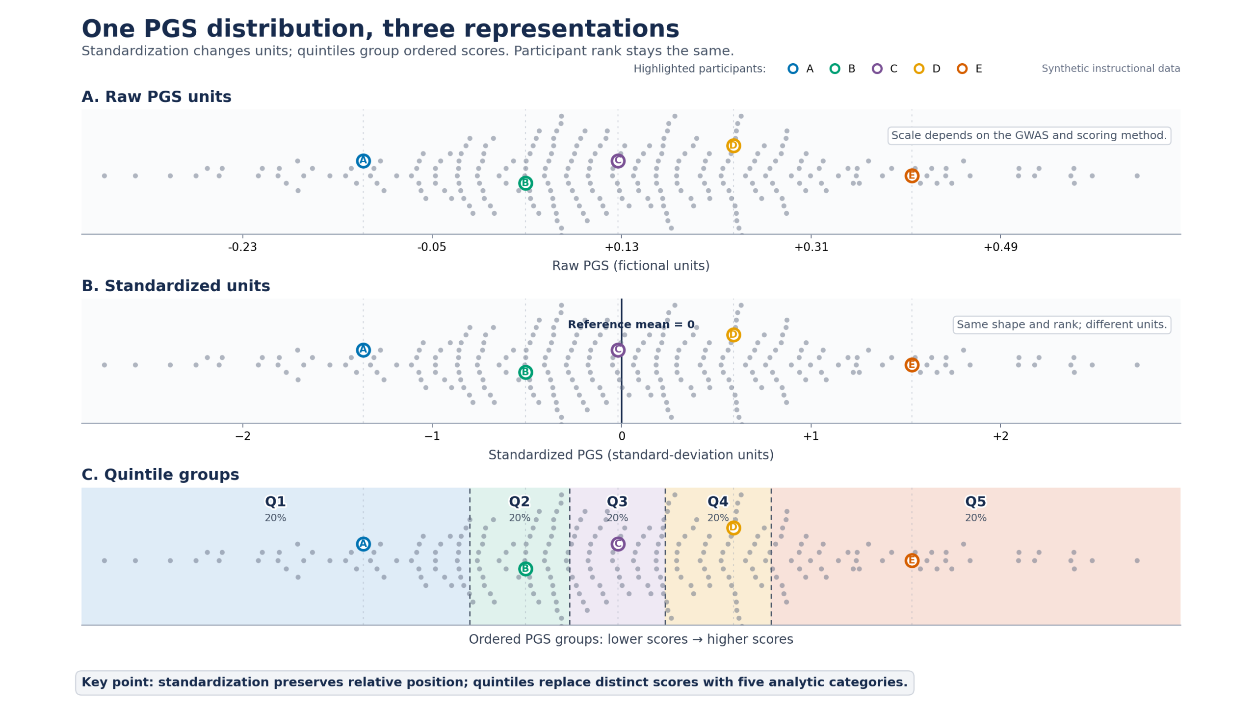
Researchers often transform a PGS so that a stated reference sample has a mean of 0 and a standard deviation of 1. The result is a standardized score, or z-score.
A standardized PGS of +1 is one standard deviation above the mean of that reference sample. A score of −1 is one standard deviation below it. Positive and negative values mean above and below the reference mean. They do not mean genetically good and bad, healthy and unhealthy, or protected and at risk.
Standardization changes the units in which the score is expressed. It does not add information, strengthen the association with an outcome, or improve predictive performance. A standardized score of +1 also does not state the probability that an outcome will occur. Formal calculation and interpretation of z-scores continue in Exercise 5 and Lab 5.
5.3 Percentiles and quantile groups
Several related terms describe a participant’s position within a score distribution:
- A z-score measures distance from the reference mean in standard-deviation units.
- A percentile describes relative rank within a reference distribution.
- A quantile group is created by ordering scores and dividing them into groups.
- A quintile is one of five groups, while a decile is one of ten.
A participant at the 90th percentile has a score at or above approximately 90% of the reference distribution. This does not mean that the participant has a 90% probability of experiencing the outcome.
Percentiles and quantile assignments depend on the reference population. The same raw score could occupy a different percentile in another sample. Quantile boundaries are analytic choices, not biological divisions between kinds of people. Turning a continuous PGS into groups can make results easier to display, but it also discards differences among participants within each group.
5.4 Distribution shape
PGS distributions are often approximately bell-shaped because each score combines many small contributions. Approximate normality should nevertheless be inspected rather than assumed. Sample selection, allele frequencies, missing genomic information, quality-control rules, and scoring decisions can all affect the observed distribution.
Standardization does not make a variable normally distributed. It changes the center and scale while preserving the distribution’s basic shape and the ordering of participants.
5.5 Outcome gradients across PGS groups
Researchers may compare an outcome across PGS quantiles. The general term for this display is an outcome gradient by PGS quantile. The narrower term risk gradient is appropriate only when the vertical axis shows an outcome probability or prevalence.
To interpret a gradient, first identify both axes. The horizontal axis should indicate the ordered PGS groups. The vertical axis might show prevalence, probability, rate, or a mean outcome. Then examine the group sizes and uncertainty around each estimate.
Ask whether the pattern is monotonic, meaning that the outcome consistently increases or decreases across the ordered groups. Also inspect the absolute size of the differences. A steadily rising line can represent very small differences. Finally, determine whether the estimates are raw or adjusted, which variables were included in any adjustment, and whether the score was evaluated in data independent of its discovery GWAS.
5.6 Group gradients and individual overlap
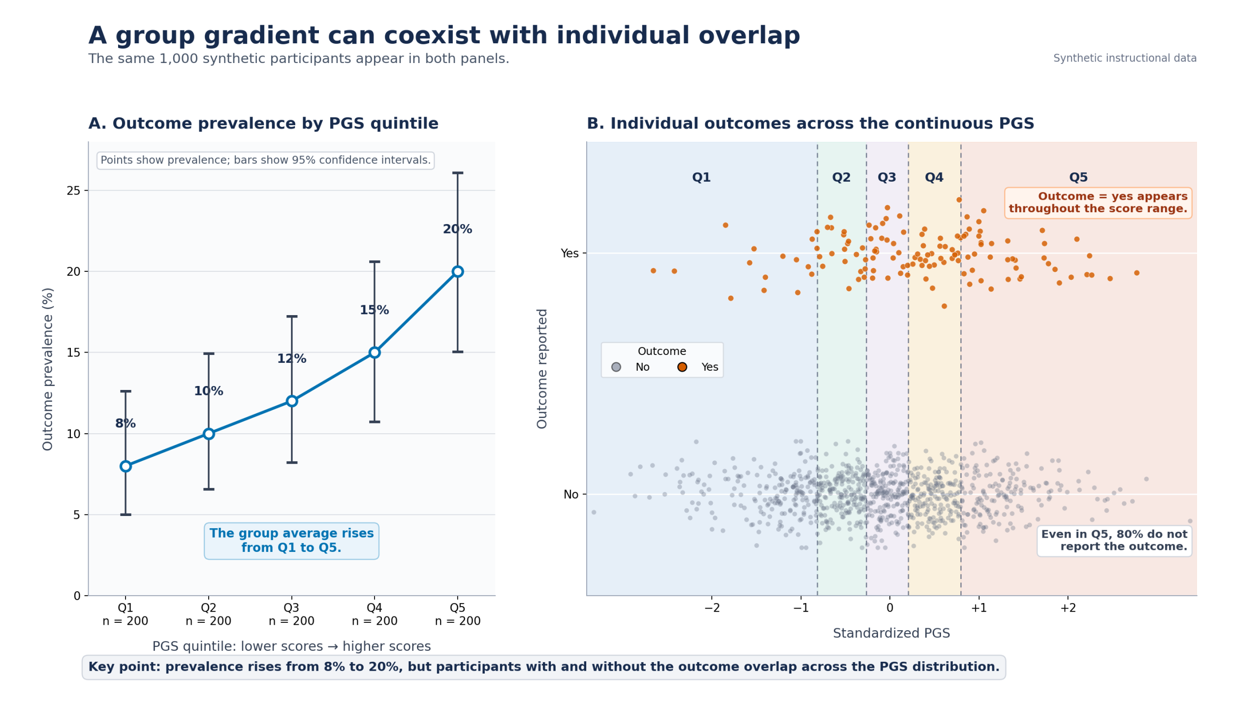
The most important limitation of a quantile plot is that it displays group averages. A rising average can coexist with extensive overlap among individuals.
For example, a high-PGS quintile may have a greater prevalence of an outcome than a low-PGS quintile. Many people in the high group may still not experience the outcome, while some people in the low group may experience it. Developmental and environmental conditions remain important, and the outcome’s base rate affects the absolute differences between groups.
Grouping can also make a weak continuous association appear more sharply separated because variation within each group is hidden. The group pattern describes an average relationship. It does not determine any participant’s outcome.
5.7 Recognizing different performance questions
No single statistic establishes whether a PGS is “effective.” Different measures answer different questions:
- Incremental R² asks how much additional variation in a continuous outcome is explained after adding the PGS to a baseline model.
- An odds ratio per standard deviation describes how outcome odds differ with a one-SD score difference. Odds are not the same as probability.
- Discrimination asks how well predictions distinguish participants with and without an outcome.
- Calibration asks whether predicted probabilities agree with observed probabilities.
- Absolute risk is the estimated probability of an outcome in a specified population and time period.
Prediction performance is multidimensional: association, explained variation, discrimination, calibration, and absolute risk answer different questions (Steyerberg et al., 2010; Lewis & Vassos, 2020).
Statistical bridge: Distributions are models
A probability distribution is a model for how values or events arise under specified assumptions. A binomial distribution can model how many people in a pair experience an outcome when a probability and independence assumption are specified. A normal distribution can provide a reference model for an approximately bell-shaped continuous variable. A Poisson distribution can model counts of events occurring within a fixed interval under specified conditions.
Choosing a familiar distribution is not enough. Researchers must ask whether its assumptions fit the process and data being studied. Exercise 5 and Lab 5 provide the formal instruction and computational applications.
6. Why genomic prediction changes across populations and contexts
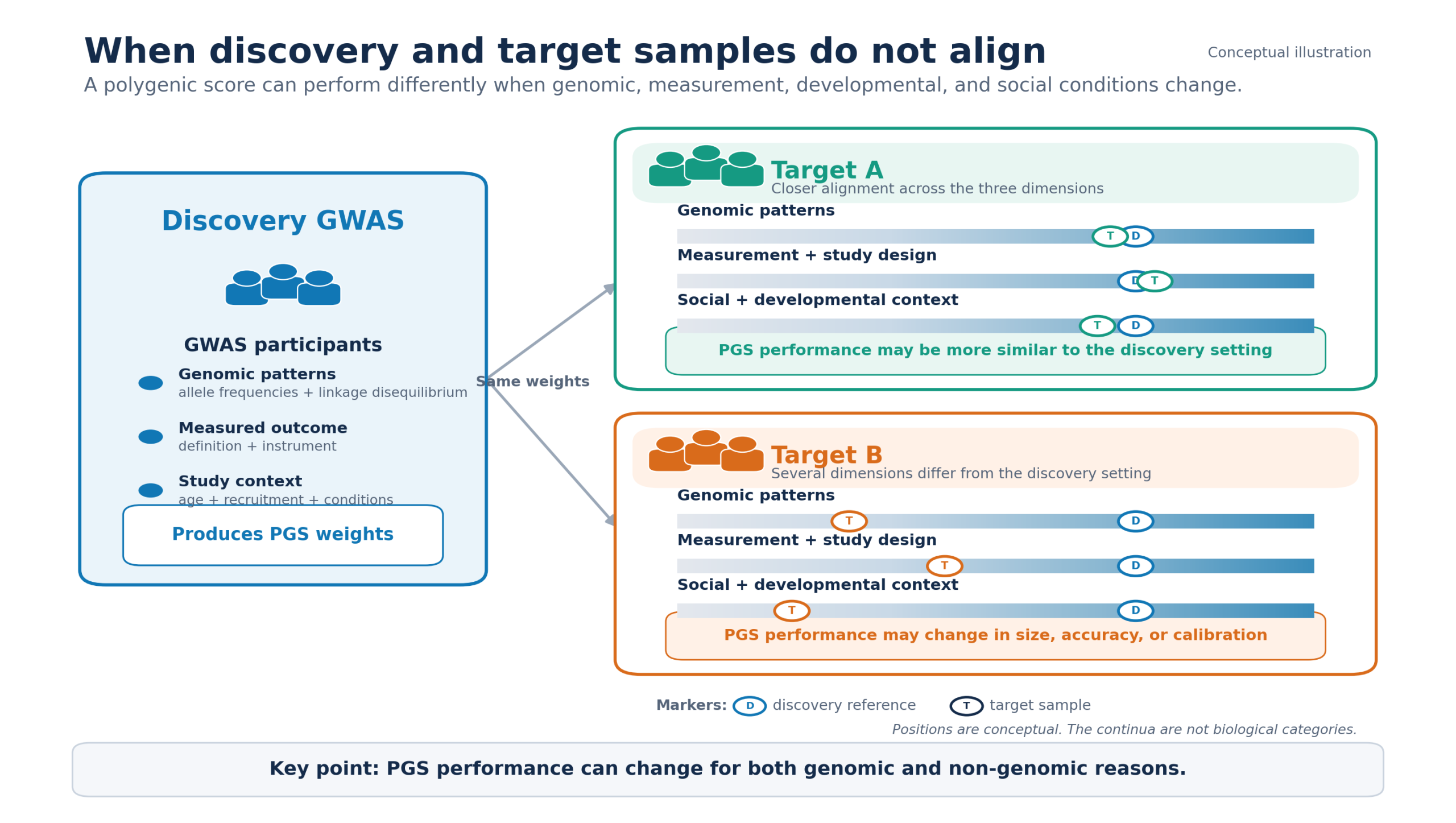
A polygenic score does not have one fixed level of predictive performance. Its performance depends on how well the data used to construct the score align with the people and conditions in which it is evaluated. This alignment involves genomic patterns, but it also involves measurement, study design, development, and social context.
6.1 Discovery-target mismatch
Recall the distinction between the two samples:
- The discovery sample supplies the GWAS estimates used as PGS weights.
- The target sample contains the participants for whom the PGS is calculated and evaluated.
Differences between them can be organized into three categories.
1. Genomic alignment. Discovery and target samples may differ in patterns of genomic similarity, allele frequencies, or linkage disequilibrium. Because nearby variants can be correlated differently across populations, a variant that serves as a useful marker in one sample may carry less information in another. Differences in genotyping platforms, imputation, and quality-control procedures can also affect which variants are available and how accurately they are measured.
2. Measurement and design alignment. Studies may use different outcome definitions, measurement instruments, recruitment procedures, or inclusion criteria. One study might measure cannabis-use frequency, while another measures cannabis use disorder. Samples may also differ in sex or gender composition and outcome prevalence. Even if the same PGS is calculated correctly, it may not perform identically when the evaluation outcome differs from the outcome studied in the discovery GWAS.
3. Social and developmental alignment. The meaning and expression of a measured outcome may change across age, developmental period, and social or environmental conditions. Access to substances, adult monitoring, stress exposure, health care, legal conditions, and opportunities for use can all differ across settings.
These categories frequently overlap. PGS portability should therefore not be reduced to a question about ancestry alone.
6.2 Population structure and genetic ancestry
Human genomic variation is continuous and overlapping. People do not fall into a small number of sharply separated genetic types. However, migration, geographic separation, reproduction, and other population histories have produced patterns of genomic similarity.
Genetic ancestry is a statistical description based on genomic data, the variants examined, the comparison samples, and the reference populations selected by researchers. It is not a complete or permanent description of a person’s identity.
As introduced in Section 3, genetic principal components summarize selected patterns of genomic similarity. Researchers may use them to account for population structure or describe variation within a sample. Neither ancestry estimates nor principal components measure race, racism, ethnicity, culture, or lived social conditions. Their interpretation depends on how they were created and why they were included (National Academies of Sciences, Engineering, and Medicine, 2023).
6.3 Race, ethnicity, and ancestry are not interchangeable
Race and ethnicity are socially and historically constructed categories. They can be connected to identity, community, culture, discrimination, political history, and unequal access to resources. Genetic ancestry, by contrast, summarizes statistical patterns in genomic variation.
Race should not be used as a substitute for genetic ancestry. Genetic ancestry should also not be used as a substitute for social experience. For example, an ancestry estimate cannot measure exposure to racism, neighborhood conditions, cultural practices, or access to treatment.
Researchers should explain why each population descriptor is included, how it was obtained, and what it represents. When a social process is relevant to the research question, it should be measured as directly as possible rather than treated as if a genomic variable captures it.
6.4 Portability and inequity
PGS generally performs best in populations that are well represented in the discovery GWAS. Performance can decline as genomic similarity between discovery and target participants decreases, although the size and pattern of that decline vary across traits and methods (Ding et al., 2023).
Historically narrow discovery samples can therefore produce unequal predictive performance. Simply increasing the total sample size does not solve this problem if the additional participants come from populations already well represented. Representation concerns who is included, how they are sampled, what is measured, and whether the resulting score is evaluated across relevant settings.
Unequal performance can distribute errors, benefits, and harms unequally. These consequences become especially important if a PGS informs screening, treatment decisions, resource allocation, or public claims about population differences. A technical limitation can become an ethical problem when the people receiving the least accurate predictions also bear the greatest consequences of error (Martin et al., 2019).
6.5 Gene-environment interaction
A gene-environment interaction, abbreviated G×E, occurs when the association between inherited differences and an outcome varies across environmental conditions. For example, a PGS-outcome association might be stronger, weaker, or expressed differently under different levels of stress, adult monitoring, opportunity, substance availability, or access to support.
This does not mean that an environment simply “activates a gene.” Both genomic and environmental measures are complex, and an observed interaction remains a statistical pattern. Studying G×E requires researchers to measure both the PGS and the environmental condition explicitly.
6.6 Gene-environment correlation
Gene-environment correlation, abbreviated rGE, refers to situations in which inherited tendencies become statistically associated with environments. Three commonly recognized forms are shown below (Plomin, DeFries, & Loehlin, 1977).
| Form | How the association develops | Addiction-relevant illustration |
|---|---|---|
| Passive rGE | Caregivers provide both inherited variation and aspects of the rearing environment. | Caregivers transmit tendencies related to behavioral regulation while also providing households with more or less structure. |
| Evocative rGE | A person’s characteristics elicit responses from other people. | A youth who behaves impulsively receives increased monitoring from adults. |
| Active rGE | People select or create environments related to their tendencies. | A sensation-seeking youth seeks novelty-oriented peers and activities. |
These pathways are not claims that environments are genetically determined. Families, institutions, peers, policies, and chance events continue to shape what environments are available. An association between a PGS and an outcome may partly reflect family or social pathways rather than a direct biological effect. Environmental measurements are therefore still necessary.
6.7 Family-level and contextual processes
Parental genotypes can be associated with environments that parents provide to their children. Research has even found associations between children’s outcomes and parental alleles that the children did not inherit, illustrating a possible indirect family pathway (Kong et al., 2018).
As a result, a PGS association measured between families may combine direct and indirect processes. Social stratification can also produce associations among genomic patterns, educational opportunities, neighborhood conditions, and health outcomes. The observed association alone cannot reveal which pathway produced it.
Within-family PGS analyses and advanced causal-genetic models can help investigate some of these questions, but they are beyond DSARM 1. The essential lesson is that a PGS is embedded in families, populations, measurements, and social contexts. Its meaning and performance cannot be interpreted from genomic information alone.
7. Governance and responsible genomic research
A 2026 New York Times investigation traced the misuse of restricted data from two major studies of children: the Philadelphia Neurodevelopmental Cohort and the ABCD Study. The Philadelphia case provides the clearest example of how a governance failure can become a scientific one.

References
References
ABCD Study. (n.d.-a). Genetics. Retrieved August 28, 2026, from https://docs.abcdstudy.org/latest/documentation/non_imaging/gn.html
ABCD Study. (n.d.-b). Letter to ABCD participants and parents. Retrieved August 28, 2026, from https://abcdstudy.org/data_safety/
ABCD Study. (n.d.-c). Open science. Retrieved August 28, 2026, from https://abcdstudy.org/open-science/
ABCD Study. (n.d.-d). Release 7.0. Retrieved August 28, 2026, from https://docs.abcdstudy.org/latest/documentation/release_notes/7_0.html
Broad Institute. (2017, August 14). Explainer: Genome-wide association studies. https://www.broadinstitute.org/visuals/explainer-genome-wide-association-studies
Choi, S. W., Mak, T. S.-H., & O’Reilly, P. F. (2020). Tutorial: A guide to performing polygenic risk score analyses. Nature Protocols, 15(9), 2759–2772. https://doi.org/10.1038/s41596-020-0353-1
Ding, Y., Hou, K., Xu, Z., Pimplaskar, A., Petter, E., Boulier, K., Privé, F., Vilhjálmsson, B. J., Olde Loohuis, L. M., & Pasaniuc, B. (2023). Polygenic scoring accuracy varies across the genetic ancestry continuum. Nature, 618(7966), 774–781. https://doi.org/10.1038/s41586-023-06079-4
Kong, A., Thorleifsson, G., Frigge, M. L., Vilhjálmsson, B. J., Young, A. I., Thorgeirsson, T. E., Benonisdottir, S., Oddsson, A., Halldorsson, B. V., Masson, G., Gudbjartsson, D. F., Helgason, A., Bjornsdottir, G., Thorsteinsdottir, U., & Stefansson, K. (2018). The nature of nurture: Effects of parental genotypes. Science, 359(6374), 424–428. https://doi.org/10.1126/science.aan6877
Lambert, S. A., Gil, L., Jupp, S., Ritchie, S. C., Xu, Y., Buniello, A., McMahon, A., Abraham, G., Chapman, M., Parkinson, H., Danesh, J., MacArthur, J. A. L., & Inouye, M. (2021). The Polygenic Score Catalog as an open database for reproducibility and systematic evaluation. Nature Genetics, 53(4), 420–425. https://doi.org/10.1038/s41588-021-00783-5
Lewis, C. M., & Vassos, E. (2020). Polygenic risk scores: From research tools to clinical instruments. Genome Medicine, 12, Article 44. https://doi.org/10.1186/s13073-020-00742-5
Martin, A. R., Kanai, M., Kamatani, Y., Okada, Y., Neale, B. M., & Daly, M. J. (2019). Clinical use of current polygenic risk scores may exacerbate health disparities. Nature Genetics, 51(4), 584–591. https://doi.org/10.1038/s41588-019-0379-x
McIntire, M. (2026, January 24). Genetic data from over 20,000 U.S. children misused for “race science.” The New York Times. https://www.nytimes.com/2026/01/24/us/children-genetics-race-science.html
National Academies of Sciences, Engineering, and Medicine. (2023). Using population descriptors in genetics and genomics research: A new framework for an evolving field. The National Academies Press. https://doi.org/10.17226/26902
National Human Genome Research Institute. (2020, August 17). Genome-wide association studies fact sheet. https://www.genome.gov/about-genomics/fact-sheets/Genome-Wide-Association-Studies-Fact-Sheet
National Human Genome Research Institute. (2023, June 27). DNA sequencing fact sheet. https://www.genome.gov/about-genomics/fact-sheets/DNA-Sequencing-Fact-Sheet
Plomin, R., DeFries, J. C., & Loehlin, J. C. (1977). Genotype-environment interaction and correlation in the analysis of human behavior. Psychological Bulletin, 84(2), 309–322. https://doi.org/10.1037/0033-2909.84.2.309
Poore, H. E., Chatzinakos, C., Leger, B., Gonzalez, J., Mallard, T. T., Aliev, F., Hatoum, A., Waldman, I. D., Sanchez-Roige, S., Palmer, A. A., Harden, K. P., Dick, D. M., & Barr, P. B. (2026). Multivariate genetic analyses of 2.2 million individuals reveal broad and substance-specific pathways of addiction risk. Nature Mental Health, 4(4), 582–593. https://doi.org/10.1038/s44220-026-00608-6
Steyerberg, E. W., Vickers, A. J., Cook, N. R., Gerds, T., Gonen, M., Obuchowski, N., Pencina, M. J., & Kattan, M. W. (2010). Assessing the performance of prediction models: A framework for traditional and novel measures. Epidemiology, 21(1), 128–138. https://doi.org/10.1097/EDE.0b013e3181c30fb2
Uban, K. A., Horton, M. K., Jacobus, J., Heyser, C., Thompson, W. K., Tapert, S. F., Madden, P. A. F., & Sowell, E. R. (2018). Biospecimens and the ABCD study: Rationale, methods of collection, measurement and early data. Developmental Cognitive Neuroscience, 32, 97–106. https://doi.org/10.1016/j.dcn.2018.03.005
U.S. Government Accountability Office. (2025). Human genomic data: HHS could better track use of foreign testing entities and strengthen oversight of security measures (GAO-25-107377). https://www.gao.gov/products/gao-25-107377
Wand, H., Lambert, S. A., Tamburro, C., Iacocca, M. A., O’Sullivan, J. W., Sillari, C., Kullo, I. J., Rowley, R., Dron, J. S., Brockman, D., Venner, E., McCarthy, M. I., Antoniou, A. C., Easton, D. F., Hegele, R. A., Khera, A. V., Chatterjee, N., Kooperberg, C., Edwards, K., … Wojcik, G. L. (2021). Improving reporting standards for polygenic scores in risk prediction studies. Nature, 591(7849), 211–219. https://doi.org/10.1038/s41586-021-03243-6