
3 Social and Environmental Pathways, Data Quality, and Data Curation
Reading Objectives
By the end of this chapter, you should be able to:
- Describe social and environmental conditions that may be associated with adolescent substance use, including attitudes, family relationships, peers, schools, neighborhoods, and availability of substances.
- Identify examples of instruments that measure attitudinal and environmental constructs, and recognize why multiple reporters and assessment waves are used.
- Explain why data quality and transparent cleaning decisions matter before analyzing social and environmental data.
- Distinguish conceptually among MCAR, MAR, and MNAR missingness mechanisms, and understand why these labels are assumptions rather than provable facts.
- Describe the source‐to‐analytic data workflow, including identifiers, events, versions, and documentation.
- Recognize ethical implications of cleaning and interpreting social and environmental data, including risks of exclusion, over‑cleaning, stigma, privacy loss, and unsupported causal claims.
Key Terms
Attitudinal factors; data quality; environmental factors; longitudinal data; missingness (MCAR, MAR, MNAR); quality-control flags; relational data; skip logic.
3.1 Social and Environmental Pathways to Substance Use
In the 1970s and early 1980s, psychologist Bruce Alexander and colleagues used a set of animal experiments often called the Rat Park studies to challenge a simplified view of addiction as only drug-driven. Across these studies, rats housed in larger, socially enriched environments often consumed less morphine solution than rats housed in more restricted laboratory housing (Alexander et al., 1981).
Rat Park does not provide a direct explanation of human substance use, and it should not be treated as a single definitive experiment. However, it offers a useful starting question: how might social connection, stress, opportunity, and environment shape substance-related behavior?
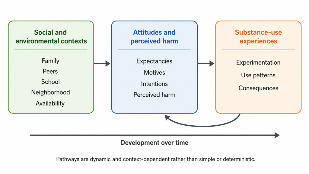
In human development, substance use is likewise associated with multiple interacting conditions. Young people’s attitudes, family relationships, peer networks, school experiences, neighborhood conditions, and access to substances can shape opportunities, expectations, stressors, and supports. These conditions do not determine any individual’s outcome, but they help researchers investigate why pathways into and away from substance use differ across people and over time.
Researchers speak of pathways because there are many possible combinations of influences rather than one deterministic sequence. A young person’s beliefs about the effects of a substance—often called attitudes or expectancies—may be shaped by what they hear from peers, family members, media, or their neighborhood. These beliefs interact with family relationships, school engagement, neighborhood safety, and access to substances. A pathway is a pattern to investigate, not a prediction about any individual.
Attitudes, Expectations, and Perceived Harm
Young people often form beliefs about substances long before they have direct experience with them. Expectancies describe beliefs about the effects a substance might have, such as feeling more relaxed or more confident. Motives capture reasons for considering or using a substance, such as coping, curiosity, or social connection. Intentions refer to plans or expectations to use a substance in the future, and perceived harm reflects beliefs about the risks of use. These constructs are latent: they cannot be directly observed but must be inferred from survey questions. Positive expectancies, low perceived harm, curiosity, and intentions may be associated with experimentation, whereas perceiving greater risk may be associated with lower willingness to initiate use. Attitudes themselves may reflect broader social norms and can change after someone gains experience with a substance.
Family Environments
Family conditions can provide support, structure, or stress. Parental monitoring refers to how much caregivers know about a young person’s activities and friends. Monitoring is meaningful only in context: it can reflect open communication and shared routines, or it may result from enforcement and surveillance. Family cohesion describes support and emotional closeness, whereas family conflict refers to recurring tension or hostility. These constructs matter because support can buffer stress and shape opportunities, while conflict or lax monitoring may coincide with riskier contexts. These conditions may be associated with different substance-use pathways, although they do not determine any individual’s outcome (Buu et al., 2009). In ABCD, measures such as the Parental Monitoring scale and the Family Environment Scale provide structured evidence of these aspects but do not capture every nuance of family life.
Peers, Social Norms, and Resistance to Influence
Peer contexts may be associated with substance use in multiple ways. Friendship networks, shared activities, and social norms can increase exposure to substances or create expectations about use (Curran et al., 1997; Dielman et al., 1990). At the same time, young people often select friends who share their interests or experiences, and both peer relationships and substance use may be shaped by family, school, or neighborhood conditions. Resistance to peer influence is a person’s ability to maintain an independent decision when feeling social pressure (Steinberg & Monahan, 2007). ABCD measures such as the Peer Behavior Profile and Resistance to Peer Influence capture aspects of peer context and the capacity to resist pressure, helping researchers examine whether peer environments are associated with substance use while recognizing their complexity.
School Engagement and Context
Schools are not just academic settings; they are major social environments. School engagement includes participation in activities, connections with teachers or classmates, interest in learning, and attendance. School context encompasses climate, relationships, resources, and policies. Engagement can provide structure and support, but it is shaped by factors beyond individual control—such as transportation, exclusionary discipline, or resource availability. Measures like the School Risk and Protective Factors scale assess how engaged students feel and whether school contexts provide support or pose risks.
Neighborhood Conditions and Substance Availability
Neighborhoods shape daily experiences through safety, social cohesion, transportation, housing, recreation, stressors, and local policies. A young person’s perception of neighborhood safety may affect where they spend time and how they experience stress. Substance availability refers to how easily substances may be obtained at home, in peer groups, in school, or in the community. Availability alone does not determine behavior; its effects depend on rules, norms, perceived harm, and individual experiences. Measures like the Neighborhood Safety/Crime Survey and Community Risk and Protective Factors describe perceived safety, community supports, and access to substances, but they should not be treated as labels for communities or residents. A neighborhood‑safety score reflects a particular perception at a particular time, not a complete description of a place.
Pathways Are Dynamic
These social and environmental factors operate together and change across development. Substance use can also alter later relationships, attitudes, and engagement. For example, experiences with a substance may influence future beliefs, peer networks, family conflict, or school involvement. Researchers therefore need longitudinal data—repeated observations of the same participants over time—to examine how attitudes, contexts, and behaviors co‑evolve. Recognizing that pathways are non‑deterministic and context‑dependent helps prevent stigma and avoids simplistic explanations for substance use.
3.2 Measurement of Attitudes and Environments
As Chapter 2 introduced, many important research constructs and concepts are not directly observed as a single raw value. Perceived harm, family cohesion, peer norms, school engagement, and neighborhood conditions are measured through indicators such as survey items, caregiver reports, administrative records, or composite scores.
The same measurement questions apply here: What was the instrument designed to capture? Who provided the information? When was it collected? How were items scored? Which responses were skipped, missing, or not applicable? Before using an attitude or environmental variable in analysis, researchers must consult the relevant documentation and interpret the value in light of how it was produced.
Indicators, Scales, and Summary Scores
Most attitudinal and environmental measures in the ABCD Study are implemented as scales consisting of multiple items. Each item provides a piece of evidence about the underlying construct. Analysts often combine items into a summary score following documented rules—sometimes reversing the direction of particular items or requiring that a minimum number of items be present. For example, a Parental Monitoring scale might ask how often a caregiver knows where the young person is, who their friends are, or what they do after school. These items are then combined into a score that represents perceived monitoring.
Multiple Reporters and Informant Differences
Many social experiences can be described from more than one perspective. Youth may be best positioned to report on private experiences, peer contexts, or perceived harm, while caregivers may provide additional information about household routines or observed behavior. Differences between youth and caregiver reports are not automatically errors or attempts to deceive. They may reflect different opportunities to observe an experience, different definitions of behaviors, privacy considerations, or changing circumstances. Consequently, analysts should avoid averaging or combining reports without a clear conceptual justification and documented scoring approach.
Examples of Measures
Table 3.1 provides examples of how latent constructs are operationalized in the ABCD Study (Lisdahl et al. 2018). It summarizes selected instruments, reporters, and broad assessment timing. This is not a complete inventory; rather, it highlights the variety of measures and the importance of consulting documentation before combining or comparing variables.
| Latent construct | Example measure | Reporter | Illustrative timing | What it captures |
| Substance expectancies | Alcohol, cannabis, nicotine, or vaping expectancy scales | Youth | Baseline and selected follow‑ups | Beliefs about effects (e.g., relaxation, social confidence, harm) |
| Motives for use | Alcohol, cannabis, nicotine, or vaping motives scales | Youth | Primarily later follow‑ups | Reasons for considering or using a substance (e.g., coping, social enhancement) |
| Intentions and perceived harm | Intention‑to‑use and perceived‑harm items | Youth | Baseline and early follow‑ups | Willingness or plans to use substances and beliefs about risks |
| Parental monitoring | Parental Monitoring scale | Youth (and sometimes caregivers) | Repeated annually | Caregiver knowledge about activities, whereabouts, and social contexts |
| Family environment | Family Environment Scale | Youth | Repeated annually | Cohesion, conflict, and aspects of household emotional climate |
| Peer context | Peer Behavior Profile; Protective Peer Network; Resistance to Peer Influence | Youth | Selected follow‑ups | Peer behavior, protective networks, and perceived ability to resist pressure |
| School context | School Risk and Protective Factors scale | Youth | Repeated annually | School environment, involvement, connection, and disengagement |
| Neighborhood and community context | Neighborhood Safety/Crime Survey; Community Risk and Protective Factors | Youth | Baseline and selected follow‑ups | Perceived safety, community supports, and access to substances |
Documentation and Interpretation
Interpreting these measures requires consulting the data dictionary, codebook, and release notes. These documents identify the item wording, response options, scoring rules, reporter, timeframe, skip logic, and versions. For example, similar constructs may be measured differently across substances or developmental stages; an alcohol expectancy scale and a cannabis expectancy scale are not automatically interchangeable. Analysts must understand which items belong to a scale, whether higher values indicate more or less of the construct, and whether any special codes represent refusal or skip responses. Only then can summary scores be responsibly used or compared across participants.
3.3 Data Quality as Concept and Practice
Attitudinal and environmental measures do not arrive in a dataset as simple, self‑explanatory facts. Before linking family, peer, school, neighborhood, and attitudinal measures to substance‑use outcomes, researchers must ask whether the available data are suitable for the question they want to answer. Data quality is not about perfection; it is about whether data are accurate, complete, consistent, timely, and relevant for a particular analysis. Large longitudinal studies almost always include incomplete records, unusual values, different reporters, technical problems, and changes across study visits. The goal is to understand what the data represent, identify limitations, and make transparent decisions about how to use them.
Inspection versus Cleaning
Data inspection means examining a dataset to understand its structure, values, patterns, and potential concerns. Analysts read the data dictionary, check ranges and variable types, count missing values, review unusual categories, and create simple summaries. Data cleaning means making documented changes based on what inspection reveals: recoding a special missing‑value code, converting a variable to the correct type, creating a quality‑control flag, or excluding records according to a justified rule. Inspection should come first. An unusual value is not automatically an error, and a blank cell is not automatically missing data. Rather than overwriting raw values, analysts should create new cleaned variables so that the original information is preserved.
Missing, Skipped, and Special‑Coded Values
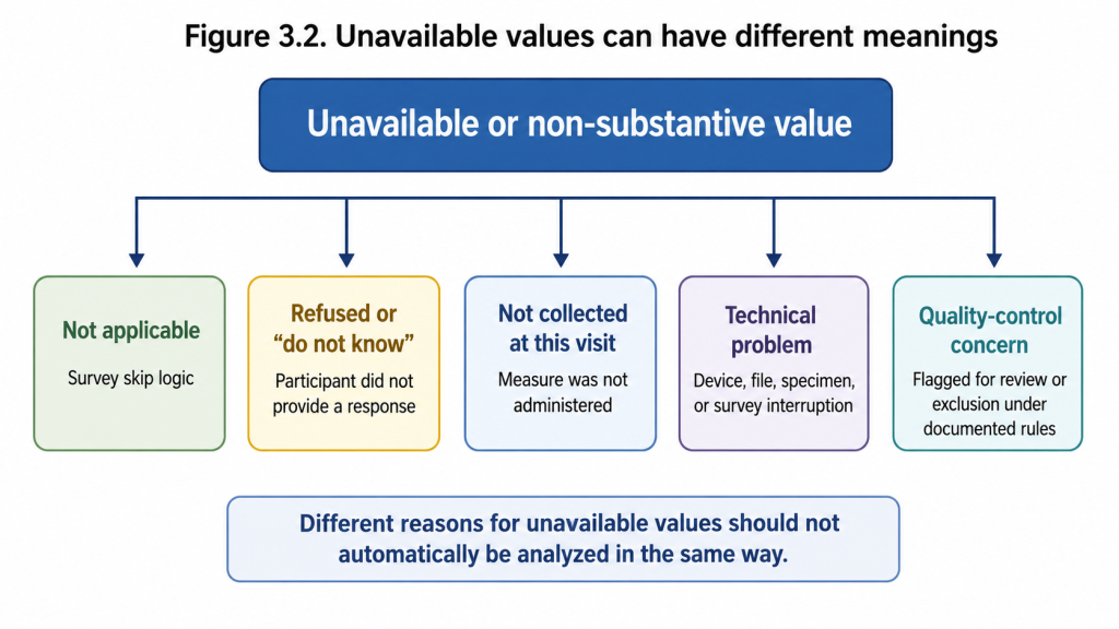
Values may be absent for many reasons: a participant may decline to answer, a question may not apply because of skip logic, a measure may not be collected at a particular visit, a specimen may be unavailable, or a technical problem may occur. These situations have different implications. For example, a past‑30‑day cannabis‑use item might be blank because a participant had never heard of cannabis (and was skipped past the question), because they declined to answer, because the measure was not collected at that visit, or because a technical failure interrupted data collection. Datasets often use numeric placeholders such as 777 or 999 to represent refusal, “do not know,” or other non-substantive responses, although the meaning of these codes varies across studies and instruments and should always be verified in the documentation (ABCD Study, n.d.). These codes must be identified and interpreted appropriately; they are not substantive high scores.
Why Missingness Matters
Missing data can distort conclusions when available records differ systematically from unavailable records. Analysts describe missingness using three conceptual categories:
- Missing completely at random (MCAR): the probability of missingness is unrelated to any observed or unobserved values. For example, a system outage might randomly affect a subset of participants.
- Missing at random (MAR): missingness is related to information observed in the dataset. For example, participants who reported transportation barriers may be less likely to return for follow‑up visits.
- Missing not at random (MNAR): missingness remains related to the unobserved value itself even after considering observed information. For example, participants with more severe substance‑related problems may be less willing to answer questions about those problems.
These categories are assumptions, not properties that can be proved from the observed dataset alone. Analysts use study design, documentation, and plausible mechanisms to decide which assumptions are reasonable. At this stage of the course, the emphasis is on identifying missing or special‑coded values, understanding why data may be unavailable, describing missingness patterns, and documenting limitations rather than performing advanced imputation.
Outliers, Unusual Values, and Quality‑Control Flags
An outlier is a value that is far from most others. Outliers may reflect data‑entry errors, incorrect units, coding problems, or genuine but uncommon observations. Unusual does not mean invalid. For example, a reported age of 450 years is almost certainly an error, whereas reporting cannabis use on every day of a 30‑day period may be uncommon but plausible and relevant. Analysts should check the documented range, units, and possible special codes before altering an outlier. Quality‑control flags signal that a response, specimen, or derived score requires caution. Flags do not automatically mean that a value should be removed; documentation may recommend retaining a flagged value for some analyses and excluding it for others.
Figure 3.3. Documented cleaning separates special codes from substantive responses
Transparent Cleaning Decisions
Cleaning decisions are analytic decisions. They can affect who remains in an analysis, how variables are distributed, and what patterns appear. A cleaning log records what issue was identified, what documentation or rule guided the decision, what change was made, how many values were affected, and whether the change altered the analytic sample. Transparent documentation allows others (and your future self) to evaluate and reproduce the analysis. It also underscores that cleaning is part of the analysis, not a hidden preliminary step. In Lab 3 you will identify special missing codes, distinguish skipped from refused responses, flag outliers, and compare distributions before and after cleaning on synthetic data.
3.4 The Source‑to‑Analytic Data Workflow
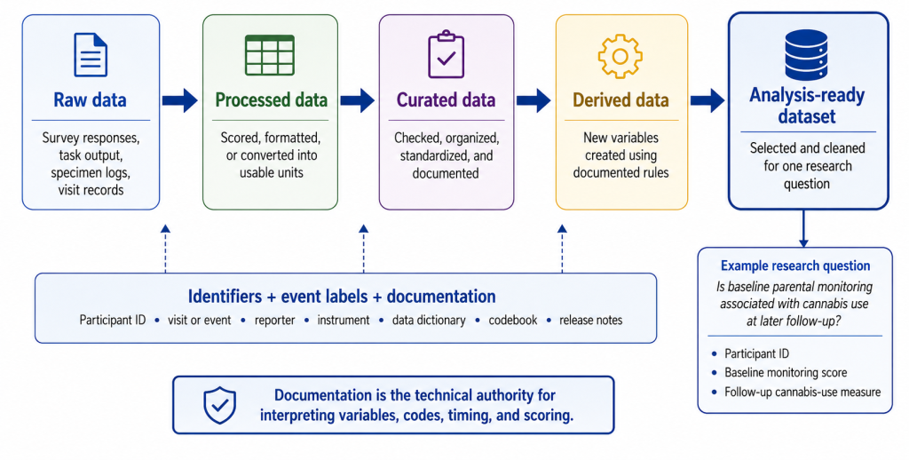
An analysis‑ready dataset is constructed, not simply downloaded. Large longitudinal studies like ABCD collect youth surveys, caregiver surveys, laboratory results, cognitive tasks, interviews, and quality‑control records across multiple visits. These raw records undergo several stages:
- Raw data: initial responses, logs, or specimens created during data collection.
- Processed data: raw records that have been scored, formatted, or converted into usable units.
- Curated data: processed data that have been organized, checked, and documented for reuse, often including standardized file and variable naming conventions, quality-control fields, and release documentation (ABCD Study, n.d.-a, n.d.-b).
- Derived data: new variables created from existing data using documented rules, such as scale scores or change‑from‑baseline values.
- Analysis‑ready data: a subset of curated and derived variables selected and cleaned for one specific research question.
Throughout this workflow, identifiers, events, and documentation guide decisions. Common identifiers include participant IDs, family IDs, study‑site IDs, visit or event labels (e.g., baseline, 1‑year follow‑up), instrument IDs, and specimen IDs. Event labels distinguish when information was collected; the same survey may be administered at multiple visits, and values cannot be interpreted without knowing the visit.
An analyst preparing a dataset to study parental monitoring and later cannabis use might need only:
- a participant identifier;
- the baseline parental‑monitoring items or score;
- a later follow‑up cannabis‑use measure;
- selected demographic or contextual variables; and
- documentation explaining the meaning, timing, and coding of each variable.
Every additional variable increases complexity and may introduce missingness or special codes that require attention. The resulting dataset is useful because it is focused, but it is also limited to the decisions made during construction.
Documentation as Technical Authority
Variable names rarely provide enough information. A variable called `parent_monitoring_total` does not tell you which items were included, who responded, whether higher scores indicate more or less monitoring, whether the score was calculated by the study or by a previous analyst, how missing items were handled, or which visit produced the value. Data dictionaries describe variables, allowable values, units, and missing‑value codes. Codebooks provide item wording, response options, scoring rules, reporters, timeframes, and skip logic. Release notes document changes across versions, corrected values, revised scoring procedures, and newly available files. Reading and citing these documents before interpretation is essential. The documentation, not a variable name, is the technical authority.
Provenance and Reproducible Cleaning
Datasets change over time as new waves are added and errors are corrected. Analysts should record the version or release used and maintain a cleaning log that notes the source table, data release, variables selected, special codes identified, transformations applied, records included or excluded, and documentation consulted. This record—sometimes called provenance—allows others to trace the history of a dataset. In Lab 3 you will practice creating a simple cleaning log using synthetic tables, joining participant and visit records, and citing documentation in code comments.
3.5 Longitudinal and Relational Data Concepts
Linking the right records is essential in longitudinal research. A participant may complete multiple surveys at multiple visits, and different pieces of information may be stored in different tables. Analysts need to understand what each row represents and how tables relate to one another.
Units of Observation and Keys
The unit of observation is the entity represented by one row in a table. One table may have one row per participant; another may have one row per participant per visit; a third may have one row per instrument or specimen. A primary key uniquely identifies each row (e.g., a participant ID in a participant table). A foreign key refers to a primary key in another table, allowing records to be linked. Relationships can be one‑to‑one (one record corresponds to one record) or one‑to‑many (one participant corresponds to many visit records). When joining tables, analysts must confirm which keys connect them and whether the relationship is one‑to‑many. Simply merging on similarly named ID columns without verifying the unit of observation can lead to duplicate or misaligned records.
Long and Wide Formats
Longitudinal datasets can be organized in long format (one row per participant per visit) or wide format (one row per participant, with separate columns for each visit). Neither format is inherently better. Long format is useful for analyzing change over time; wide format can be convenient for comparing selected time points.
Retention, Attrition, and Follow‑Up
Longitudinal studies depend on retaining participants. Retention means continuing participation across visits, whereas attrition occurs when participants leave the study or become unavailable. Missing a follow‑up visit is not necessarily the same as attrition, but both can affect available data. Participants with incomplete follow‑up data may differ systematically from those with complete records—for example, youth experiencing greater instability may have more missing visits. Analysts should examine retention patterns, document inclusion criteria, and avoid assuming that the available follow‑up sample represents the entire baseline cohort.
3.6 Ethical Issues in Cleaning and Interpretation
Data cleaning is not merely technical; it is also ethical. Decisions about which values to recode, retain, flag, exclude, or combine can affect who is represented in an analysis and what variation is visible. Removing a participant who reported cannabis use on all 30 days of a 30‑day period because it is rare would erase an important experience. Conversely, failing to recode a 999 refusal code would distort summaries. Analysts should ask: What does this value represent? Why am I changing it? Which participants are affected? Does documentation support the decision? Can another analyst reproduce the process?
Responsible Interpretation and Privacy
Social and environmental measures are context‑dependent evidence, not labels for individuals, families, schools, or communities. A neighborhood‑safety score should not be used to stigmatize a community; a family‑conflict score is not a complete description of a family. Associations between school disengagement and substance use do not establish causation. Researchers should avoid framing social conditions as individual failures and should acknowledge alternative explanations and contextual influences. When reporting results, they must respect privacy by avoiding small cells or combinations of characteristics that could identify participants. Documentation of cleaning decisions helps prevent misinterpretation and supports reproducibility.
Chapter Summary
This chapter examined how social and environmental contexts may be associated with adolescent substance use. Attitudes, expectancies, motives, intentions, perceived harm, family relationships, peer norms, school engagement, neighborhood conditions, and substance availability are latent constructs that interact in dynamic pathways. They are measured through instruments that require careful operationalization, multiple reporters, and documented scoring rules. Data quality matters because incomplete, inconsistent, or poorly documented data can distort conclusions. Analysts must inspect data, identify special codes and missingness patterns, and document cleaning decisions. An analysis‑ready dataset is constructed through curation, versioning, identifiers, event labels, and transparent provenance. Longitudinal and relational structures mean that analysts must understand units of observation, primary and foreign keys, event labels, and retention patterns. Cleaning and interpretation are ethical practices: they shape who is represented, preserve meaningful variation, and influence how communities are portrayed.
References
ABCD Study. (n.d.-a). Curation standards. Retrieved July 6, 2026, from https://docs.abcdstudy.org/latest/documentation/curation/standards.html
ABCD Study. (n.d.-b). Naming conventions. Retrieved July 6, 2026, from https://docs.abcdstudy.org/latest/documentation/curation/naming.html
Alexander, B. K., Beyerstein, B. L., Hadaway, P. F., & Coambs, R. B. (1981). Effect of early and later colony housing on oral ingestion of morphine in rats. Pharmacology Biochemistry and Behavior, 15(4), 571–576. https://doi.org/10.1016/0091-3057(81)90211-2
Buu, A., McCartan, C., Lamb, K., Benning, K., Schmidt, D., & Rothman, E. (2009). Parent, family, and neighborhood effects on the development of child substance use and other psychopathology from preschool to the start of adulthood. Journal of Studies on Alcohol and Drugs, 70(4), 489–498. https://doi.org/10.15288/jsad.2009.70.489
Curran, P. J., Stice, E., & Chassin, L. (1997). The relation between adolescent alcohol use and peer alcohol use: A longitudinal random coefficients model. Journal of Consulting and Clinical Psychology, 65(2), 130–140. https://doi.org/10.1037/0022-006X.65.2.130
Dielman, T. E., Butchart, A. T., & Shope, J. T. (1990). Structural equation model tests of patterns of family interaction, peer alcohol use, and intrapersonal predictors of adolescent alcohol use and misuse. Journal of Drug Education, 23(3), 273–316. https://doi.org/10.2190/9F1C-T4X7-9VK6-25F9
Lisdahl, K. M., Sher, K. J., Conway, K. P., Gonzalez, R., Feldstein Ewing, S. W., Nixon, S. J., Tapert, S., Bartsch, H., Goldstein, R. Z., & Heitzeg, M. (2018). Adolescent brain cognitive development (ABCD) study: Overview of substance use assessment methods. Developmental Cognitive Neuroscience, 32, 80–96. https://doi.org/10.1016/j.dcn.2018.02.007
Steinberg, L., & Monahan, K. C. (2007). Age differences in resistance to peer influence. Developmental Psychology, 43(6), 1531–1543. https://doi.org/10.1037/0012-1649.43.6.1531