
4 Behavioral Genetics and Addiction-Relevant Traits
Reading Objectives
By the end of this chapter, you should be able to:
- Distinguish externalizing and internalizing pathways associated with addiction risk.
- Compare family, adoption, classical twin, and discordant-MZ study designs.
- Explain how mental health and neurocognitive measurements become family-linked phenotypes.
- Interpret paired scatterplots and compare MZ and DZ correlations.
- Use Falconer equations to approximate and interpret A, C, and E.
Key Terms
DNA · gene · genetics · exposure · phenotype · externalizing · internalizing · familial aggregation · monozygotic (MZ) twins · dizygotic (DZ) twins · zygosity · cotwin resemblance · paired observation · additive genetic variance (A) · shared environmental variance (C) · nonshared environmental and residual variance (E) · Falconer equations · heritability · discordant-MZ design
1. Introduction
In the marshmallow test, you place one marshmallow in front of a young child and offer a choice: eat it now, or wait and receive two marshmallows later. This is the basis of a well-known study designed to assess delayed gratification. Waiting longer has also been studied as a predictor of a range later-in-life outcomes, such as impulsive tendencies (Mischel et al., 1989). However, it should be noted that more recent research has found that associations between waiting and subsequent outcomes become smaller after accounting for family and developmental conditions (Watts et al., 2018).
Externalizing vs Internalizing
Impulsivity is a construct, which we defined in Chapter 2 as an abstract and unobservable concept used to describe human mental processes, traits, or behaviors; researchers must infer these tendencies from surveys, behavioral tasks, observations, and patterns across situations. The construct of impulsivity includes acting without sufficient forethought, favoring immediate rewards, or having difficulty stopping a response.
Impulsivity is categorized within the broader construct of externalizing. Externalizing refers to outwardly expressed patterns of behavioral disinhibition. These patterns can include impulsivity, sensation seeking, rule-breaking, aggression, oppositional behavior, and difficulty controlling actions. A contrasting pathway is internalizing, which refers to distress that is directed inward, including persistent anxiety, depressed mood, worry, withdrawal, and negative affect. They exist on continua. A person can show relatively more or less of these tendencies without having a behavioral disorder.

Externalizing and internalizing are two classic pathways to substance use and addiction. For externalizing, young people who are highly sensation seeking or behaviorally disinhibited may begin experimenting with substances earlier, enter more high-risk situations, or have greater difficulty limiting use once it begins. This does not mean that impulsivity inevitably produces addiction. It means that externalizing tendencies can increase risk when they combine with substance availability, peer contexts, stress, and other conditions (Iacono et al., 2008). In contrast, a person experiencing internalizing problems may use alcohol or other substances to reduce distress, escape unwanted thoughts, or feel temporary relief. This is sometimes described as a coping or self-medication pathway (Hussong et al., 2011).
Externalizing and internalizing are not mutually exclusive boxes. The same person may experience both behavioral disinhibition and emotional distress. The pathways can also intersect. For example, negative urgency refers to a tendency to act rashly while experiencing intense negative emotion. It connects an internalizing condition, emotional distress, with an externalizing response, impulsive action.
These pathways describe patterns of risk, not predetermined routes to addiction. Most people with internalizing or externalizing tendencies do not develop a substance use disorder. Social relationships, opportunities, stressors, protective resources, substance exposure, and developmental changes all influence whether and how risk is expressed.
Where do these differences come from?
Why do people differ in impulsivity, externalizing behavior, internalizing distress, and other behavioral traits and characteristics? Chapters 1 through 3 examined how constructs are measured and how social and environmental conditions contribute to different developmental pathways. This chapter introduces another part of the question: whether inherited biological differences also contribute to variation among people.
Four terms are necessary for asking this question.
DNA is the molecule that stores biological information in cells. People receive DNA from both biological parents. A gene is a region of DNA involved in producing or regulating a biological function. Most human DNA is shared across people, but differences in DNA sequences contribute to biological variation. There is no single gene for impulsivity, internalizing, or addiction. These complex outcomes reflect many genetic differences operating through development and in combination with lived conditions.
A phenotype is an observed or derived characteristic that researchers measure and compare. Phenotypes can be physical or behavioral characteristics, like height or introversion and extroversion. Calling something a phenotype does not mean that it is fixed, purely genetic, or directly observable without measurement.
Genetics is the study of DNA, inheritance, and biological variation. When researchers ask whether a phenotype is genetically influenced, they are not asking whether genes determine an individual’s future. They are asking whether inherited differences help explain why measurements of that phenotype vary among people in a particular population and context.
An exposure is a condition, experience, or behavior whose possible relationship with an outcome is being studied. The term does not refer only to toxic chemicals. Family conditions, peer relationships, stress, neighborhood environments, and access to substances can all be exposures. Alcohol or cannabis use can also be treated as an exposure when researchers ask whether sustained use is associated with later life outcomes.
In many cases, people who share DNA often share exposures, like families and environments. Inherited tendencies may affect how people respond to the same exposure or which situations they encounter. Exposures may strengthen, weaken, or redirect the expression of inherited differences. The measurement process also affects the phenotype that researchers ultimately analyze. This makes the motivating question difficult:
How can researchers investigate whether genetic differences contribute to variation in externalizing, internalizing, and other addiction-related phenotypes when biological relatives also share important exposures and environments?
Family, adoption, and twin studies approach this problem by comparing people who differ in their expected genetic relatedness and rearing relationships. This chapter examines the logic and limitations of those comparisons. It then traces how family-linked observations become measured phenotypes, paired records, correlations, and estimates of genetic and environmental variation. We do not use a “nature vs nurture” framework, as we assume an approach that how genes and environments act together to lead to complex outcomes like addiction.
2. From Family Resemblance to Genetically Informative Designs
Behavioral genetics is a branch of science that studies the influence of genetic and environmental factors on behaviors. In the context of addiction, behavioral genetics helps identify why some individuals are more susceptible to substance use disorders than others. Foundational study designs include family, adoption, classical twin, and discordant-twin studies; each design addresses a different question, depends on different assumptions, and may represent a different population (Willoughby, Polderman, & Boutwell, 2023).
2.1 Family studies: detecting familial aggregation
A family study asks whether a diagnosis, behavior, or measured trait occurs more often, or is more similar, among relatives than would be expected in the broader population. Researchers might compare rates of alcohol use disorder among the relatives of people with and without the disorder, or examine whether parent and youth scores on addiction-relevant traits are associated.
When elevated risk or resemblance occurs within families, the outcome is said to show familial aggregation. Alcohol and other substance use disorders, including cannabis use disorder, have repeatedly been found to aggregate within families (Merikangas et al., 1998). This pattern can be scientifically and clinically informative. For example, a reported family history of alcohol or cannabis problems may help identify young people with elevated risk who could benefit from additional assessment or prevention resources.
Familial aggregation does not reveal why relatives resemble one another. Biological relatives may share inherited genetic variation, but they may also share housing, resources, stressors, substance availability, cultural practices, and patterns of family interaction. Relatives can also influence one another’s behavior. A family-history measure further depends on what the respondent knows, remembers, and is willing to report. It is therefore an imperfect indicator of familial liability, not a genetic measurement or evidence that an outcome is inherited.
2.2 Adoption studies: separating some genetic and rearing relationships
Adoption studies introduce a different comparison. An adopted person shares inherited genetics with biological relatives without sharing a household. Researchers can therefore compare resemblance with biological and adoptive relatives to investigate whether a trait follows genetic relationships, adoptive relationships, or both. However, this comparison remains observational. The design remains observational and is limited by prenatal influences, selective placement, later contact, and the limited representativeness of many adoption samples.
2.3 Classical twin studies: comparing degrees of genetic relatedness
The classical twin design compares monozygotic (MZ, or identical twins) and dizygotic (DZ, or fraternal twins) twin pairs. MZ twins develop from the same fertilized egg and share nearly all their inherited DNA. DZ twins develop from separate fertilized eggs and share, on average, approximately half of their genes, the same expected proportion as ordinary biological siblings. Both sets of twins are the same age and commonly share a household, caregivers, schools, communities, and many other features of early development.
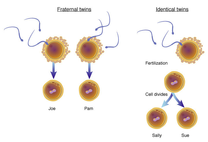
In twin studies, researchers measure the same observed traits in both members of each twin pair. Next, they estimate how strongly cotwins resemble one another. For example, imagine that MZ twins show strong consistency in smoking cannabis, if one MZ twin is a frequent smoker, then the other is too; and we find little consistency in cannabis smoking among DZ twins, if one DZ twin smokes then it has no association to smoking behaviors in the other twin. In this example, MZ twins are more highly correlated in cannabis smoking than DZ twins, and that pattern is consistent with genetic differences contributing to variation in cannabis smoking (our trait of interest). A wealth of twin studies have shown that substance use – and nearly any behavior you can name – are genetically influenced (Dick, 2021). However, twin studies do not prove that genes caused the trait. The genetic inference in twin studies depends on assumptions about relevant environmental similarity, mating patterns, measurement quality, and the comparability of the MZ and DZ samples (Rijsdijk & Sham, 2002).
2.4 Discordant-MZ studies: comparing differences within pairs
A discordant-MZ study focuses on identical twins who differ in an exposure or experience. Discordant means different within the pair. Researchers then ask whether the twins also differ on a later outcome.
For example, suppose one MZ twin has greater cannabis exposure than the cotwin. Researchers could compare the twins’ later scores on the same memory test. The analysis asks whether the twin with greater exposure also has a different memory score.
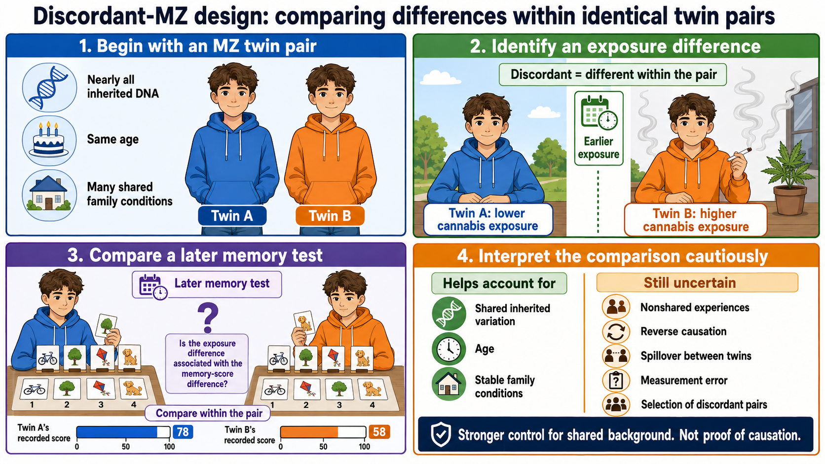
This comparison provides stronger control for shared inherited and family conditions than a comparison between unrelated participants. If the twins differ in memory scores, that difference cannot easily be attributed to characteristics that are the same for both twins.
However, MZ twins can still have different friends, stressors, illnesses, school experiences, and mental-health conditions. Any of these individual experiences could contribute to both cannabis exposure and memory performance. The memory difference could also have existed before the exposure difference, one twin’s behavior could affect the other, or imperfect measurements could make the twins appear more different or similar than they are. Only pairs that differ sufficiently in exposure are useful for the comparison, and those pairs may not represent all MZ twins.
The two twin approaches therefore answer different questions. A classical twin study compares MZ and DZ resemblance to investigate why people vary in a measured characteristic. A discordant-MZ study compares differences within MZ pairs to examine an exposure-outcome relationship while accounting for much of the twins’ shared background.
| Design | Who or what is compared? | What the comparison helps researchers examine | What remains uncertain |
|---|---|---|---|
| Family study | People from the same family compared with people from other families or the broader population | Whether a diagnosis, behavior, or trait tends to run in families | Whether the resemblance reflects inherited variation, shared environments, or both |
| Adoption study | An adopted person’s resemblance to biological relatives compared with resemblance to adoptive relatives | Whether resemblance more closely follows biological relationships, the rearing household, or both | Prenatal influences, selective placement, later contact with biological relatives, and whether adoptive families represent the broader population |
| Classical twin study | Resemblance among identical, or MZ, twins compared with resemblance among fraternal, or DZ, twins | Whether greater genetic similarity is associated with greater similarity in the measured trait in MZ twins compared to DZ twins | Whether relevant environments were equally similar for MZ and DZ twins, along with measurement and sampling limitations |
| Discordant-MZ study | Two MZ twins who differ in an exposure or trait | Whether the more-exposed twin also differs in an outcome after accounting for stable inherited differences and much of the shared family background | Individual experiences, timing, reverse causation, measurement error, and why the twins became different |
These comparisons become informative only when researchers know what was measured, how relatives were identified and linked, and which assumptions the design requires. The ABCD twin study illustrates how that evidence is produced.
3. The ABCD Twin Study as a Biomedical Data Journey
ABCD Study includes a twin subsample of 772 same-sex twin pairs (N = 1,544 youth) enrolled at ages 9–10 at baseline. ABCD intentionally oversampled twins at four sites with established twin registries and expertise (University of Colorado Boulder, University of Minnesota, Virginia Commonwealth University, Washington University in St. Louis) using state birth records and standardized recruitment (Iacono et al., 2018). Zygosity (MZ vs DZ) was inferred from genomic markers (e.g., the Smokescreen array; Uban et al., 2018), improving classification accuracy. The twin cohort—while broadly similar to the full ABCD sample—tends to include families with somewhat higher parental education and income and lower racial/ethnic diversity (Iacono et al., 2018). All procedures were IRB-approved (Auchter et al., 2018), with parental consent and child assent.
3.1 Data Architecture and Family-Linked Records
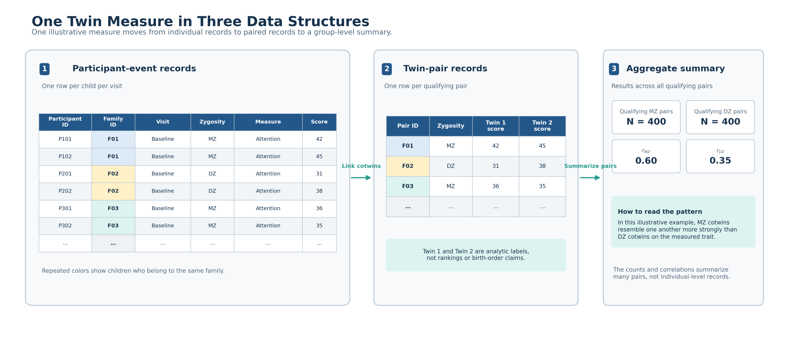
Twin data are hierarchical because individual participants belong to larger groups. Each child belongs to a twin pair and family, and each family is associated with a study site. The same participant may also contribute records at multiple visits. Consequently, in an ABCD-like dataset, two rows belonging to the same family are related observations, not two unrelated people sampled independently.
In a participant-level longitudinal table, one row might represent one child at one visit. That row would need a participant identifier, family identifier, event or visit label, measure name, and score version. A paired-participant identifier connects that child to the cotwin, while a zygosity field indicates whether the pair is classified as MZ or DZ. Current ABCD documentation provides fields such as gn_y_genrel_id__fam for genetically related family groups, gn_y_genrel_id__paired__01 for paired participants, and gn_y_genrel_zyg__01 for relationship classification (ABCD Study genetics documentation).
| Stage | Physical and operational infrastructure | Data architecture | Governance and provenance |
|---|---|---|---|
| Recruit and collect | Twin registries and birth records, four specialized research sites, staff, study visits, digital instruments, and biospecimens | Participant, family, birth-set, site, visit, instrument, and score-version records | Parent consent, youth assent, approved recruitment procedures, and standardized data collection |
| Process and link | Genotyping laboratories, equipment, computational pipelines, and quality-control procedures | Genomic relatedness and zygosity classifications; linked family records using fields such as gn_y_genrel_id__fam, gn_y_genrel_id__paired__01, and gn_y_genrel_zyg__01 (ABCD genetics documentation) |
Secure data transfer, access controls, quality review, and documentation of the data release and processing history |
| Analyze and share | Research teams and approved computing environments | Participant records reorganized into pair-level datasets; separate MZ and DZ correlations; ACE model estimates; aggregate Twin Hub results | Controlled access to individual-level data, aggregate public sharing, and interpretation appropriate to the sample and data release (ABCD data-access documentation) |
Relatedness methods, variable names, scoring procedures, and available records can change across releases, making the release and processing history essential parts of data provenance.
4. Selected mental health and neurocognitive measures
Modules 2 and 3 introduced selected instruments and variables from the ABCD Substance Use data domain. These included youth and caregiver reports, structured interviews, summary variables, and toxicology measures used to study substance exposure and substance-related outcomes. This chapter broadens our view of the ABCD data.
Section 3 introduced the Genetics domain through the ABCD twin sample. This section turns to selected measures from two additional domains: Mental Health and Neurocognition. Recall that a data domain is a broad organizational category that groups related instruments, procedures, and variables.
The ABCD Study includes many measures within each domain. We will examine only a small set:
- Child Behavior Checklist Internalizing and Externalizing Problems
- UPPS-P Negative Urgency
- a selected NIH Toolbox neurocognitive score
These measures also connect the chapter’s theories to its twin comparisons. Once a characteristic has been recorded or derived, researchers can use it as a phenotype in comparisons among ABCD participants, including twins. A phenotype might be a caregiver-reported behavioral score, a youth-reported tendency, or a cognitive-task score.
4.1 Mental health measures: reports of emotions and behavior
The ABCD Mental Health domain includes instruments used to study emotions, behavior, personality, psychiatric symptoms, and family mental-health history. Some instruments are completed by youth, some by caregivers, and some by teachers. These different sources are useful because no single respondent has complete access to a young person’s experiences.
Two measures in this module connect directly to the internalizing and externalizing pathways introduced at the beginning of the chapter.
The Child Behavior Checklist, or CBCL, is completed by a parent or caregiver about the participating youth. It asks about emotional and behavioral difficulties and produces several dimensional scores. A dimensional score represents the extent to which reported behaviors or symptoms are present. It is not simply a yes-or-no classification.
The CBCL Internalizing Problems score summarizes caregiver reports of anxiety, depressed mood, withdrawal, somatic complaints, and other forms of inward-directed distress. The Externalizing Problems score summarizes reports of rule-breaking, aggression, and other outwardly expressed behavioral difficulties. Because both scores come from the same instrument and respondent, they provide a useful measured contrast between the two theoretical pathways discussed in the introduction (Barch et al., 2018).
The scores nevertheless reflect a caregiver’s observations. Caregivers may notice disruptive behavior more readily than private worries or emotions. They may also differ in how they interpret an item, how often they observe a behavior, and what they consider unusual. A lower internalizing score could mean that a youth is experiencing little distress, but it could also mean that the distress was not visible to the caregiver. The score represents documented responses to a set of items, not complete access to the youth’s mental life. Scoring rules are also part of the measurement process. Individual CBCL responses are combined into syndrome and summary scores, which depends on item responses, missingness, scoring rules, and the version of the released data being used (ABCD Mental Health documentation).
The UPPS-P Impulsive Behavior Scale for Children provides a different kind of mental-health measure. In the modified ABCD version, youth complete 20 self-administered questions that contribute to several impulsivity subscales. This module focuses on negative urgency, the tendency to act rashly when experiencing intense negative emotion.
Negative urgency is narrower than the broad CBCL Externalizing Problems score. It describes a particular form of impulsive action under distress. The negative emotion identifies the context in which rash action occurs; it does not make negative urgency a measure of internalizing problems. Negative urgency is most directly relevant to impulsivity and externalizing risk, although emotional distress may help activate the behavior.
The CBCL and UPPS-P therefore differ in at least three ways. They represent different constructs, use different respondents, and apply different scoring procedures. A caregiver reports observations of the youth for the CBCL, while the youth reports on their own tendencies for the UPPS-P. Youth self-report provides access to experiences that caregivers may not observe, but it also depends on self-knowledge, item interpretation, memory, comfort, and willingness to report.
Mental-health measures require careful and respectful interpretation. A CBCL or UPPS-P score should not be treated as the identity of a participant. Researchers should describe a participant as having a recorded score, not as being an “externalizing child” or an “impulsive person.” The ABCD documentation also cautions that mental-health items and scores may function differently across cultural and social groups. Scores derived from research instruments should not automatically be interpreted as clinical diagnoses, and apparent group differences should not be assumed to represent inherent differences between groups (ABCD Mental Health documentation).
4.2 Neurocognitive measures: performance under specified conditions
Neurocognitive tasks are used in the behavioral sciences to assess mental processes using structured tests, rather than surveys. The ABCD Neurocognition domain includes standardized tasks intended to measure aspects of attention, executive function, memory, language, learning, and processing speed.
At baseline, the ABCD neurocognition battery included seven NIH Toolbox Cognition tasks administered using an iPad. Examples include the Flanker Inhibitory Control and Attention Test, Picture Sequence Memory Test, List Sorting Working Memory Test, and Pattern Comparison Processing Speed Test. The battery was selected to support prospective research on cognitive development, vulnerabilities that precede substance use, and possible cognitive changes associated with later substance exposure (Luciana et al., 2018).
A task is designed to emphasize a particular form of performance. For example, the Flanker task is intended to measure attention, cognitive control, executive function, and the inhibition of an automatic response. List Sorting is intended to measure working memory, while Picture Sequence Memory is intended to measure episodic memory. These labels describe the intended constructs, but performance is not produced by a single ability in isolation.
A participant’s score may also be affected by comprehension, fatigue, sleep, nutrition, motivation, familiarity with digital devices, distraction, temporary stress, and the testing environment. Practice can matter when participants complete related tasks at multiple visits. A cognitive-task score is therefore evidence of performance on a particular task under particular conditions. It is not a direct measurement of a fixed intellectual capacity. Additionally, the ABCD documentation specifically recommends considering socioeconomic experiences, transient performance conditions, normative reference samples, and whether measures function comparably across groups when interpreting neurocognitive data (ABCD Neurocognition documentation).
4.3 From recorded measures to phenotypes
Chapter 2 introduced the sequence through which an abstract construct becomes an analytic variable:
Construct → instrument or task → respondent or administration → recorded response → scoring process → analytic variable → interpretation
The measures discussed this section share this sequence. Externalizing behavior becomes a recorded phenotype only after researchers select an instrument, obtain caregiver responses, apply scoring rules, and choose a particular score. Negative urgency becomes a recorded phenotype through a different instrument, respondent, and scoring process. Neurocognitive performance becomes a phenotype through a standardized task and its scoring algorithm. In the next section, we discuss methods for estimating the extent to which a given phenotype is genetically influenced.
5. Seeing and summarizing cotwin resemblance
Section 4 introduced several phenotypes that can be compared across ABCD participants. In a twin analysis, the next question is whether the two members of a twin pair tend to receive similar scores on the selected phenotype.
Researchers examine this question in two related ways. A paired scatterplot shows the pattern of cotwin scores, while a correlation summarizes the strength and direction of their association. The new conceptual step is understanding that each point represents one twin pair, not one individual participant.
5.1 Reading a twin-pair scatterplot
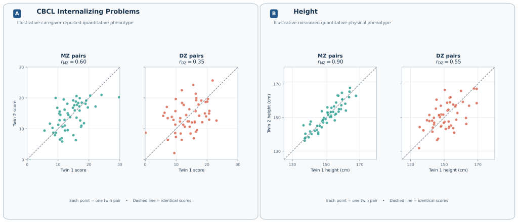
Figure 4.4 compares cotwin resemblance in two quantitative phenotypes: CBCL Internalizing Problems and height. Each phenotype has separate scatterplots for MZ and DZ pairs. Within each plot, Twin 1’s value appears on the horizontal axis and Twin 2’s value appears on the vertical axis. Each point represents one twin pair. Twin 1 and Twin 2 are analytic labels, not rankings or indicators of importance. A pair can be included only when both cotwins have qualifying values for the same phenotype, score version, and visit (no missing data for either twin).
5.2 Resemblance and exact agreement are different
The dashed 1:1 line shows where cotwins with identical values would fall. Points closer to the line indicate smaller within-pair differences.
Correlation describes a different feature: how consistently the two cotwins’ values vary together across pairs. The correlation coefficient, (r), ranges from (-1) to (1). A value closer to (1) indicates a stronger positive linear association. Cotwin values can be strongly correlated without being identical.
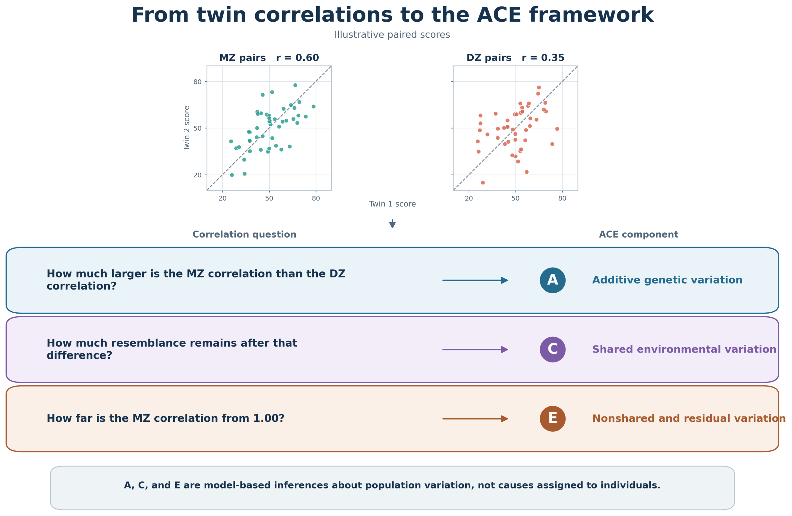
In the illustrative CBCL example, rMZ = .60 and rDZ = .35. In the height example, rMZ = .90 and rDZ = .55. MZ cotwins show stronger resemblance than DZ cotwins for both phenotypes. Classical twin reasoning depends on comparing the MZ and DZ correlations for the same phenotype. Neither correlation should be interpreted alone.
5.3 Inspect the pattern before interpreting the correlation
A correlation reduces a paired-score pattern to one number. Researchers should first inspect:
- the direction, form, and strength of the pattern;
- unusual observations that might strongly affect the correlation;
- the range and concentration of the scores; and
- overlapping points that may hide multiple pairs.
The type of phenotype matters. Height usually varies across a broad continuous range. A behavioral-problem score may contain many zeros or repeated values. Scores concentrated near the minimum produce a floor effect, scores concentrated near the maximum produce a ceiling effect, and scores covering only a narrow interval have a restricted range. Each can make resemblance difficult to evaluate.
Measurement error, temporary conditions, missing cotwin values, and pair-selection rules can also change the observed correlation. A weak correlation may therefore reflect the distribution or measurement of the phenotype, not a complete absence of cotwin resemblance.
5.4 What a twin correlation does and does not establish
Three distinctions are essential when interpreting twin correlations.
- Correlation is not agreement. Cotwin scores can follow a strong linear pattern without being identical or close to the 1:1 line.
- Correlation is not causation. Cotwin resemblance does not identify why the twins are similar. Resemblance could reflect inherited differences, shared exposures, shared developmental conditions, or other processes.
- Correlation is not a complete measurement judgment. A high correlation does not establish that the instrument measured the intended construct completely, comparably, or without bias.
If MZ cotwins are more highly correlated than DZ cotwins, the pattern is consistent with inherited differences contributing to variation in the recorded phenotype. It does not prove that genes caused the phenotype, and it does not show how much of any individual participant’s score came from genes or environments. The next section explains this interpretation in more detail.
6. From twin correlations to the ACE framework
MZ and DZ correlations describe cotwin resemblance. The ACE framework is a simplified statistical model that divides observed variation into additive genetic, shared environmental, and nonshared environmental components (Neale & Cardon, 1992; Rijsdijk & Sham, 2002). It divides variation in a recorded phenotype into three modeled components: additive genetic variance, shared environmental variance, and nonshared environmental and residual variance.
ACE does not directly observe genetic or environmental causes. It uses differences in resemblance across many twin pairs to estimate how much variation may be associated with each component.
6.1 Three sources of modeled variation
Suppose researchers measure an externalizing score in a sample of twins. Some children receive relatively high scores, some receive relatively low scores, and many fall between them. The spread of these recorded scores represents variation in the phenotype.
A: Additive genetic variance
The A component represents variation associated with inherited genetic differences whose effects combine additively. An additive effect is one in which contributions from inherited variants accumulate. A does not identify a particular gene, and it does not include every possible genetic process. It represents additive genetic variation under the assumptions of the model.
C: Shared environmental variance
The C component represents environmental variation that contributes to cotwin resemblance. Household conditions, family resources, neighborhood context, or shared experiences could contribute to C when they make cotwins more similar on the recorded phenotype.
C is not a complete measurement of “the family environment.” The same experience may affect two children differently. If cotwins respond differently to a family transition, for example, the resulting difference would not contribute to C merely because the event occurred within their shared household.
E: Nonshared environmental and residual variance
The E component represents variation that contributes to differences within MZ pairs. It can include person-specific experiences, different responses to shared experiences, temporary assessment conditions, measurement error, and other unexplained variation.
For example, one cotwin might be tired during a cognitive assessment while the other is well rested. A caregiver might also interpret similar behaviors differently for the two children. These influences can reduce observed cotwin resemblance and contribute to E.
A, C, and E are model components, not substances or percentages located inside an individual. When standardized, the components sum to 1.00 apart from rounding. They describe modeled variation among people in a particular population and measurement context.
6.2 Extending the correlation comparison
The ACE framework extends the MZ-DZ correlation comparison by asking three questions, summarized in Figure 4.5.
.
Not every correlation pattern fits the basic ACE model comfortably. If both correlations are low, restricted variation, measurement limitations, or substantial within-pair differences may be involved. If the DZ correlation is less than half the MZ correlation, nonadditive genetic processes or other model complications may need to be considered. These comparisons do not establish causation by themselves. Their interpretation depends on the phenotype, sample, expected genetic relationships, environmental assumptions, and statistical model (Rijsdijk & Sham, 2002).
6.3 Falconer equations
The Falconer equations provide a classroom approximation of A, C, and E using the two observed correlations (Falconer & Mackay 1996) :
A ≈ 2(rMZ − rDZ)
C ≈ 2rDZ − rMZ
E ≈ 1 − rMZ
The difference between the MZ and DZ correlations is doubled to approximate A because MZ twins share about twice as much segregating genetic variation as DZ twins, on average. C is estimated from the remaining resemblance shared by DZ twins after accounting for the approximate additive genetic contribution. E is estimated from the difference between perfect MZ resemblance and the observed MZ correlation.
Consider the illustrative correlations introduced in Section 5:
rMZ = .60 rDZ = .35
The approximate additive genetic component is:
A ≈ 2(.60 − .35) = 2(.25) = .50
The approximate shared environmental component is:
C ≈ 2(.35) − .60 = .70 − .60 = .10
The approximate nonshared environmental and residual component is:
E ≈ 1 − .60 = .40
The three estimates sum to 1.00:
.50 + .10 + .40 = 1.00
A bounded interpretation would be:
Under the simplified ACE model, approximately 50% of the modeled variation in this recorded phenotype was attributed to additive genetic differences, 10% to shared environmental differences, and 40% to nonshared environmental, measurement, and residual differences in the illustrative population and measurement context.
This does not mean that 50% of any participant’s phenotype is genetic. The calculation describes variation among people, not the composition of an individual, explained further in the next section.
Finally, Falconer equations express the central logic of the classical twin comparison, but professional research analyses generally use formal variance-component models (Rijsdijk & Sham, 2002).
7. What heritability means and what the evidence permits us to say
In the basic ACE model, the standardized A component is commonly interpreted as heritability, often written (h2). Heritability describes how much variation in a recorded phenotype is statistically attributed to additive genetic differences under a particular model.
This definition is more limited than everyday statements such as “intelligence is genetic” or “addiction runs in families.” Responsible interpretation requires specifying the population, developmental period, measurement, environments represented, and model used to produce the estimate.
7.1 Heritability is a population parameter
A population parameter describes a characteristic of a defined population. Researchers generally do not observe the true population value directly. They estimate it from a sample.
Heritability concerns:
- variation among people;
- in a specified population;
- during a specified developmental period;
- across the environments represented in that population;
- for a particular recorded phenotype;
- under a particular design and analytic model.
Heritability is therefore not a permanent number attached to a trait that can be applied to any sample or population. Heritability can also change when environments change. If a population contains little environmental variation, inherited differences may account for a larger proportion of the remaining variation. If environmental conditions become more varied, the estimated proportion attributed to genetic differences may decrease. The underlying biological processes do not have to change for the heritability estimate to change (Visscher et al., 2008).
7.2 Assumptions and sources of uncertainty
Twin estimates depend on assumptions. These assumptions do not automatically invalidate the design, but they define what conclusions the evidence can support.
- Relevant environmental comparability. Classical twin reasoning assumes that environmental similarity related to the phenotype does not differ between MZ and DZ pairs in a way that fully explains their difference in resemblance. It does not assume that MZ and DZ twins experience identical environments.
- Mating patterns. The simple model relies on expectations about genetic resemblance among DZ twins. If biological parents resemble one another on characteristics related to the phenotype, the expected genetic covariance relevant to that phenotype may differ from the simplest model.
- Comparable and adequate measurement. The phenotype must be measured sufficiently consistently across cotwins and zygosity groups. Informant differences, unreliable scores, altered task versions, administration changes, or ceiling effects can change the correlations and resulting estimates.
- Selection and attrition. Families who enroll, remain in a longitudinal study, and provide complete scores for both cotwins may differ from families who do not. The qualifying analytic pairs may therefore represent a selected portion of the original sample.
- Model identification. The basic MZ and DZ comparison can distinguish only the components supported by the available family relationships and assumptions. It does not discover every biological, developmental, and environmental process that contributes to the phenotype.
- Sampling uncertainty. Correlations and ACE components are estimates. Different samples drawn from the same population would not produce exactly the same values. Confidence intervals and other uncertainty estimates help show the range of values reasonably compatible with the data.
The ACE framework separates variation into genetic and environmental components for analysis, but genetic and environmental processes do not operate independently. In gene–environment interaction (G×E), the relationship between inherited differences and an outcome varies across environmental conditions. In gene–environment correlation (rGE), inherited tendencies become associated with the environments people receive, evoke, or select. These processes complicate attempts to interpret A, C, and E as completely separate causal forces. Chapter 5 develops these concepts further.
7.3 Reporting heritability responsibly
Family and twin evidence can easily be overstated, particularly when research concerns children, mental health, substance use, or socially marginalized populations.
Responsible reporting should name the recorded phenotype, population, developmental period, design, model, and uncertainty. It should use population-level language such as “consistent with genetic influence” or “modeled variation attributed to A.” Heritability estimates should not be presented as percentages inside an individual, evidence of genetic destiny, or explanations for differences between social groups.
The ABCD Study’s responsible-use guidance emphasizes interpretation within the relevant social and environmental context. Responsible reporting is part of scientific validity, not an optional step after analysis. In Chapter 5, we examine issues of responsible use and misuse of genetic data in research.
References
Auchter, A. M., Hernandez Mejia, M., Heyser, C. J., Shilling, P. D., Jernigan, T. L., Brown, S. A., Tapert, S. F., & Dowling, G. J. (2018). A description of the ABCD organizational structure and communication framework. Developmental Cognitive Neuroscience, 32, 8–15. https://doi.org/10.1016/j.dcn.2018.04.003
Barch, D. M., Albaugh, M. D., Avenevoli, S., Chang, L., Clark, D. B., Glantz, M. D., Hudziak, J. J., Jernigan, T. L., Tapert, S. F., Yurgelun-Todd, D., Alia-Klein, N., Potter, A. S., Paulus, M. P., Prouty, D., Zucker, R. A., & Sher, K. J. (2018). Demographic, physical and mental health assessments in the Adolescent Brain and Cognitive Development study: Rationale and description. Developmental Cognitive Neuroscience, 32, 55–66. https://doi.org/10.1016/j.dcn.2017.10.010
Dick, D. M. (2021). The child code: Understanding your child’s unique nature for happier, more effective parenting. Avery.
Falconer, D. S., & Mackay, T. F. C. (1996). Introduction to quantitative genetics (4th ed.). Longman.
Hussong, A. M., Jones, D. J., Stein, G. L., Baucom, D. H., & Boeding, S. (2011). An internalizing pathway to alcohol use and disorder. Psychology of Addictive Behaviors, 25(3), 390–404. https://doi.org/10.1037/a0024519
Iacono, W. G., Heath, A. C., Hewitt, J. K., Neale, M. C., Banich, M. T., Luciana, M. M., Madden, P. A., Barch, D. M., & Bjork, J. M. (2018). The utility of twins in developmental cognitive neuroscience research: How twins strengthen the ABCD research design. Developmental Cognitive Neuroscience, 32, 30–42. https://doi.org/10.1016/j.dcn.2017.09.001
Iacono, W. G., Malone, S. M., & McGue, M. (2008). Behavioral disinhibition and the development of early-onset addiction: Common and specific influences. Annual Review of Clinical Psychology, 4, 325–348. https://doi.org/10.1146/annurev.clinpsy.4.022007.141157
Luciana, M., Bjork, J. M., Nagel, B. J., Barch, D. M., Gonzalez, R., Nixon, S. J., & Banich, M. T. (2018). Adolescent neurocognitive development and impacts of substance use: Overview of the Adolescent Brain Cognitive Development (ABCD) baseline neurocognition battery. Developmental Cognitive Neuroscience, 32, 67–79. https://doi.org/10.1016/j.dcn.2018.02.006
McGue, M., Osler, M., & Christensen, K. (2010). Causal inference and observational research: The utility of twins. Perspectives on Psychological Science, 5(5), 546–556.
Merikangas, K. R., Stolar, M., Stevens, D. E., et al. (1998). Familial transmission of substance use disorders. Archives of General Psychiatry, 55(11), 973–979.
Mischel, W., Shoda, Y., & Rodriguez, M. I. (1989). Delay of gratification in children. Science, 244(4907), 933–938. https://doi.org/10.1126/science.2658056
Neale, M. C., & Cardon, L. R. (1992). Methodology for genetic studies of twins and families. Kluwer Academic Publishers. https://doi.org/10.1007/978-94-015-8018-2
Rijsdijk, F. V., & Sham, P. C. (2002). Analytic approaches to twin data using structural equation models. Briefings in Bioinformatics, 3(2), 119–133.
Uban, K. A., Horton, M. K., Jacobus, J., Heyser, C., Thompson, W. K., Tapert, S. F., Madden, P. A. F., Sowell, E. R., & the Adolescent Brain Cognitive Development Study. (2018). Biospecimens and the ABCD study: Rationale, methods of collection, measurement and early data. Developmental Cognitive Neuroscience, 32, 97–106. https://doi.org/10.1016/j.dcn.2018.03.005
Visscher, P. M., Hill, W. G., & Wray, N. R. (2008). Heritability in the genomics era: Concepts and misconceptions. Nature Reviews Genetics, 9(4), 255–266. https://doi.org/10.1038/nrg2322
Watts, T. W., Duncan, G. J., & Quan, H. (2018). Revisiting the marshmallow test: A conceptual replication investigating links between early delay of gratification and later outcomes. Psychological Science, 29(7), 1159–1177. https://doi.org/10.1177/0956797618761661
Willoughby, E. A., Polderman, T. J. C., & Boutwell, B. B. (2023). Behavioural genetics methods. Nature Reviews Methods Primers, 3.