9 Chapter 9: Analysis & Results

Learning Objectives

• Understand the difference between data analysis and data science in health research.
• Learn about the various statistical tests used in data analysis and how to choose the appropriate test based on the research question and data type.
• Recognize the importance of interpreting statistical results correctly, including understanding absolute vs. relative risk, correlation vs. causation, and confounding vs. controlling.
• Explore the applications of data science in health research, including predictive modeling, clustering, and natural language processing.
• Gain insight into qualitative data analysis methods, including category construction and coding techniques.

Key Terms

• Data Analysis: The process of examining, cleaning, transforming, and modeling data to discover useful information, inform conclusions, and support decision-making.
• Data Science: An interdisciplinary field that uses scientific methods, processes, algorithms, and systems to extract knowledge and insights from data.
• Statistical Tests: Procedures used in statistics to make inferences or decisions about population parameters based on sample data, often involving the calculation of a test statistic and a p-value.
• Absolute Risk vs Relative Risk: Absolute risk is the actual probability of an event occurring in a population, while relative risk is the ratio of the probability of an event occurring in one group compared to another.
• Correlation vs Causation: Correlation is a measure of the strength and direction of the relationship between two variables, while causation implies that changes in one variable directly cause changes in another.

Introduction

This chapter describes data analysis and data science in health research, exploring how these methodologies are employed to extract meaningful insights from data and drive informed decision-making. It begins with an exploration of data analysis, focusing on its importance in drawing conclusions and making predictions based on existing data. The chapter then transitions to data science, highlighting its broader scope that includes predictive modeling and data-driven decision-making. Through examples from ABCD research, the chapter illustrates the application of statistical methods in investigating associations between various factors and outcomes.

Data Preparation: Handling Missing Values & Outliers

Before beginning data analysis, researchers must make a plan for missing or invalid data and outliers. This is especially true in large and complex datasets like those from the ABCD study, as missing values and outliers as they can significantly impact the study’s results and conclusions.

Missing Values

Missing data can arise for various reasons in health research, including non-response, loss to follow-up, or errors in data collection. The approach to handling missing data depends largely on the nature and pattern of the missingness.

Why Address Missing Values?

• Bias Reduction: Proper handling of missing data can reduce sample bias, or at least highlight the bias for more accurate interpretation of results.
• Improved Accuracy: Accurate imputation of missing values can lead to more precise estimates of statistical parameters.
• Increased Statistical Power: By effectively dealing with missing data, you maintain a larger sample size, enhancing the statistical power of your study (introduced in Chapter 6: Sampling).

Addressing Missing Values

Here are common methods to address missing data:

• Listwise Deletion: This involves removing any cases (rows) that have missing values. While simple, this method can lead to bias if the missing data are not completely random.
• Imputation: Imputation replaces missing values with substituted values. The substitution can be as simple as the mean, median, or mode (for more robust measures), or as complex as using predictions from a regression or machine learning model. Multiple imputation is a sophisticated technique that creates several imputed datasets and combines the results to account for the uncertainty of the imputations.
• Using a Model to Account for Missingness: Some statistical models, like certain types of regression, can be adapted to directly handle missing data by maximizing the likelihood function for the observed data. For example, if you’re dealing with missing MRI data that is not random but correlated with participants’ health status, using multiple imputation can help model this relationship and reduce bias.

Outliers

Outliers are extreme values that differ significantly from other observations. They can be legitimate or due to measurement or input errors, and their handling is crucial as they can distort the results.

Why Address Outliers?

• Reduce Skewness: Outliers can skew the distribution of the data, leading to misleading analysis.
• Enhance Model Accuracy: Removing or adjusting outliers can improve the accuracy of regression and other statistical models.
• Increase Robustness: Handling outliers properly increases the robustness of the statistical results, making them more reliable under various conditions.

Addressing Outliers

Before deciding how to handle outliers, you need to identify them. Techniques include:

• Statistical Tests: Such as Grubb’s test or Dixon’s test for identifying single outliers.
• Visual Inspection: Box plots, scatter plots, and histograms can help visualize and identify outliers.
• Standard Deviation: Observations more than 2 or 3 standard deviations from the mean can be considered outliers.
• Interquartile Range (IQR): Values below Q1 – 1.5 * IQR or above Q3 + 1.5 * IQR are often regarded as outliers.

After identifying outliers, researchers must address them, and these are common methods to address outliers:

• Exclude: Remove outliers if they are errors or if you’re certain they are not valuable for your analysis.
• Transform: Apply a transformation (log, square root) to reduce the impact of extreme values.
• Cap: Winsorizing, or capping, involves replacing outliers with the nearest value that is not an outlier.
• Modeling: Use robust statistical methods like robust regression that can accommodate outliers.

Researchers must document their approach to handling missing data and outliers clearly. This includes a description of the rationale for the chosen method. This enhances the reproducibility of the study (discussed towards the end of this chapter).

Considerations with ABCD Data

When working with the Adolescent Brain Cognitive Development (ABCD) Study or similar large longitudinal datasets, special attention must be given to how outliers are handled, as they can significantly influence the results and interpretations of the research (Saragosa-Harris, et al., 2022). The ABCD Study, like many large-scale studies, includes a diverse range of data points, some of which are extreme values or outliers. These outliers can belong to different categories (Saragosa-Harris, et al., 2022):

• Error Outliers: These are data points that reflect errors in the dataset. Researchers should be cautious and conservative when identifying these outliers, considering exclusion only if there is clear evidence of errors in administering, reporting, or transcribing the data. The ABCD Study’s working groups perform quality control checks for impossible data points before each release, which helps reduce the occurrence of these error outliers.
• Valid/Interesting Outliers: In large datasets, some extreme values are actually of interest because they represent unique, but valid, variations within the population. These outliers can be particularly valuable in studies like ABCD, where the goal is to explore a wide range of behavioral and health outcomes across a diverse population. Eliminating these interesting outliers could mean losing critical information that could contribute to understanding atypical behaviors or conditions.
• Influential Outliers: These are extreme values that are accurate but might unduly influence the statistical models without being of theoretical interest to the specific research question. It’s important to identify these outliers and decide on a strategy—such as robust statistical methods or tailored modeling approaches—to mitigate their influence without losing valuable information.

Planning for Outliers with ABCD

Researchers need to plan carefully for how to detect and handle outliers in ABCD data (Saragosa-Harris, et al., 2022):

• Detection: Standard methods like using 3 standard deviations from the mean may not be suitable due to the large size of the dataset. Alternative methods, including multivariate approaches and robust statistical tests, should be considered based on the research question and the characteristics of the data.
• Documentation: It is crucial to document the methods used for outlier detection and handling. This documentation should include the rationale for chosen methods and any implications for the analysis.
• Impact Assessment: Consider performing sensitivity analyses to understand how different approaches to handling outliers affect the results. This can provide insights into how robust the findings are to the presence of outliers.

Data Analysis vs Data Science

Data analysis is primarily concerned with extracting insights from existing data. Google Career Certificate programs define data analysis as “the collection, transformation, and organization of data in order to draw conclusions, make predictions, and drive informed decision-making” (2021). For instance, statistical analysis might be used to evaluate the effectiveness of a new medication in a clinical trial, or to analyze epidemiological data to identify risk factors for a particular disease.

Data science encompasses a broader scope, including data analysis, predictive modeling, and data-driven decision-making. Google defines data science as, “creating new ways of modeling and understanding the unknown by using raw data” (Google Career Certificates, 2021). Data science leverages tools and techniques such as machine learning and “big data” technologies. In health research, this might involve developing predictive models to forecast disease outbreaks based on environmental and health data, or applying machine learning algorithms to analyze medical imaging data or genome sequences for early detection of diseases.

While data analysis focuses on finding answers to existing questions by creating insights from data sources, data science goes a step further by creating new questions and exploring innovative ways to model and understand data. Both play vital roles in advancing health research and improving patient outcomes, but they do so through different approaches and methodologies.

Data Analysis in Health Research

Overview of Regression, Correlation, and Comparison Tests

Data analysis in health research includes both descriptive statistics and inferential statistics, which are used to test research questions and hypotheses. There are three primary types of inferential statistical tests used in this domain:

• Regression Analysis: This type of analysis is used to understand the relationship between independent (predictor) and dependent (outcome) variables and to make predictions. Regression can show how the dependent variable changes when any one of the independent variables is varied, while the other independent variables are held fixed.
• Correlation: This measures the strength and direction of the linear relationship between two variables without assuming a dependent relationship. It is crucial for determining how variables are related without implying causation.
• Comparison Tests: These tests are used to identify and estimate quantitative differences between two or more groups. This involves starting with a null hypothesis (discussed in Chapter 3), which typically states that no difference exists between groups or conditions.

Regression Analysis

Regression analysis is a statistical tool that models the relationship between two or more variables. It allows researchers to examine how changes in one or more independent variables affect the dependent variable. Regression is used in health research for predicting outcomes and understanding the factors that influence those outcomes.

• Linear Regression: This is the simplest form of regression analysis and is used when the relationship between the variables is linear. Linear regression fits a straight line to the data, which can be used to predict the value of the dependent variable based on the value of the independent variable. For instance, linear regression could be used to predict systolic blood pressure based on age.
• Multiple Regression: This extends linear regression to include more than one independent variable. It helps in understanding the relationship between a dependent variable and several independent variables. For example, multiple regression could be used to determine how age, weight, and smoking status together affect the risk of developing cardiovascular diseases.
• Nonlinear Regression: When the relationship between the dependent and independent variables is not linear, nonlinear regression is used. This type of analysis can fit complex models to data, such as exponential and logarithmic relationships.
• Logistic Regression: This is used when the dependent variable is categorical (e.g., success/failure or yes/no). Logistic regression estimates the probability of a certain class or event existing. For example, it could be used to predict the likelihood of a patient having a heart attack within the next year based on their cholesterol levels and age.

Correlation

Correlation measures the strength and direction of the linear relationship between two variables. It is represented by the correlation coefficient, which ranges from -1 to +1.

• Pearson’s Correlation: This measures the linear relationship between two variables, providing a coefficient that denotes the strength and direction of this linear relationship.
• Spearman’s Rank Correlation: This is a non-parametric measure of rank correlation, used when the data do not necessarily come from a bivariate normal distribution, and it measures the strength and direction of the monotonic relationship between two variables.

Comparison Tests

Comparison tests evaluate whether the differences between groups are statistically significant, based on the observed data and the null hypothesis.

• T-Tests: These are used to compare the means of two groups. For instance, an independent t-test compares the means of two independent groups to determine if there is evidence that the associated population means are significantly different. A paired t-test, on the other hand, compares the means of the same group or items under two separate scenarios.
• ANOVA (Analysis of Variance): This is used to compare the means of three or more groups. For example, ANOVA could be used to determine if there is any significant difference in the mean systolic blood pressure across different age groups.
• Non-Parametric Tests: When the data do not meet the assumptions required for parametric tests, non-parametric tests like the Mann-Whitney U test (for two independent groups) or the Kruskal-Wallis test (for three or more groups) are used.

Choosing Statistical Tests

The research question and/or hypothesis will typically guide determination of the type of statistical test(s) to use in data analysis. This implies that the main statistical tests in data analysis are determined at the research question / hypothesis generation phase of research planning (Chapters 3 & 4). There are two main considerations in selecting statistical tests to answer a research question, how variables are measured and the assumptions of the statistical test.

Measurement of Variables

The measure of variables refers to their level of measurement, introduced in the chapter on Instrumentation (Chapter 7). A brief recap of levels of measurement:

• Categorical Data: Variables can be measured categorically, in which values correspond to groups, such as gender (male, female) or blood type (A, B, AB, O). It can be nominal (no inherent order, like race and ethnicity) or ordinal (with a natural order, like small, medium, large).
• Continuous Data: This type of data can take any value within a range and is often measured. Examples include height, weight, and temperature. It can be interval (where the difference between values is meaningful, but there’s no true zero, like temperature in Celsius) or ratio (where both differences and ratios are meaningful, and there is a true zero, like weight or height).

Assumptions of Statistical Test

Each statistical test comes with specific assumptions that must be satisfied for the test results to be valid:

• Normality: Many parametric tests assume that the data are normally distributed.
• Homogeneity of Variance: Assumes that data groups have the same variance.
• Independence: Assumes that the observations are independent of each other.

For example, parametric tests like t-tests and ANOVAs are appropriate for continuous data that meet assumptions of normality and homogeneity of variances. When these assumptions are not met, researchers should consider non-parametric alternatives like the Mann-Whitney test or Kruskal-Wallis test.

Identifying Statistical Tests to Use

Choosing the right statistical test involves matching the research question and the data’s characteristics with a suitable test, considering both the type and assumptions of the data:

• For Comparing Groups: Use t-tests for comparing means between two groups, or ANOVA for more than two groups, when data meet parametric assumptions.
• For Examining Relationships: Employ regression analysis to explore relationships between variables. Simple linear regression could be used to assess how one continuous variable predicts another, while logistic regression might be suitable for predicting a binary outcome from one or more predictor variables.

Ultimately, researchers choose statistical tests based on the study design and the literature supporting the use of particular data analysis tools to answer a research question. At beginner to intermediate levels in research and data analysis, there are a variety of tables and flowcharts that can be help match research questions and statistical tests, such as this one from the UCLA Advanced Research Computing group.

For example, below are common comparison tests which test group differences in means, such as in experimental designs with treatment and control groups.

Table 7: Example of Uses of Comparison Tests
Statistical Test	Independent Variable	Dependent Variable	Research Question Example
Paired t-test	One variable with two categories (e.g., pre-test vs post-test)	One quantitative variable in which groups come from the same population	Does a new pain medication significantly reduce pain scores compared to baseline scores in patients with chronic back pain?
Independent t-test	One variable with two categories (e.g., treatment vs control group)	One quantitative variable in which groups come from the different populations	Is there a difference in average weight loss between individuals following a low-carb diet and those following a low-fat diet for a period of 12 weeks?
ANOVA	One variable with two or more categories (e.g. multiple treatments vs control)	One continuous variable	What is the difference in average recovery times among patients undergoing three different types of physical therapy for knee injuries?

Additionally, below are common regressions tests which test correlations (associations) among variables.

Table 8: Example of Uses of Regression Tests
Statistical Test	Independent Variable	Dependent Variable	Research Question Example
Simple Linear Regression	One continuous independent variable	One continuous independent variable	How does age predict systolic blood pressure in adults?
Multiple Linear Regression	Two or more continuous independent variables	Two or more continuous independent variables	How do age and BMI together predict cholesterol levels in adults?
Logistic Regression	One or more independent variables (can be continuous or categorical)	Categorical dependent variable with only two categories (e.g., success/failure, yes/no)	How do smoking status and age predict the likelihood of heart disease in adults?

However, interpreting the results of statistical tests, such as the one introduced above, is not a straightforward process.

Caution in Interpretation of Results

These are three important considerations when interpreting the results of the above-mentioned statistical methods and tests:

Absolute vs Relative Risk

Absolute risk refers to the actual risk of an event happening in a specific population. For example, if 2 out of 100 people develop a disease, the absolute risk is 2%. Relative risk compares the risk in two different groups. For example, if the risk of developing a disease is 4% in one group and 2% in another, the relative risk is 2 (4% divided by 2%). This means the first group has twice the risk of the second group. Many studies report relative risk metrics rather than absolute risk (Attia 2018), which has potential to be misleading or be misinterpreted by the public, as described in Figure 10.

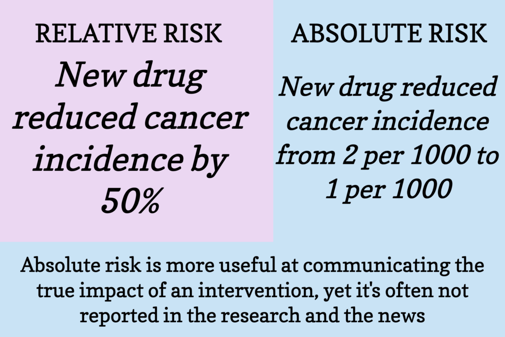
Figure 10: Relative vs Absolute Risk. Image Credit: Attia, P. 2018.

Correlation vs Causation

Another concern in the interpretation of quantitative data is the conflation of correlation and causation, which happens to some of the most trained researchers. Correlation is a statistical relationship between two variables. For example, there might be a correlation between ice cream sales and temperature, meaning they tend to occur together. However, correlation does not imply that one causes the other. Causation means that one variable directly influences another. In the case of smoking and lung cancer, extensive research has established that smoking causes lung cancer. Misinterpreting correlation as causation can lead to incorrect conclusions.

In most instances, health researchers seek to establish causations, to identify the root causes of health conditions and states. Recall that clinical trials approximate causation by randomly assigning participants to treatment and control groups, which helps to control for confounding variables and biases (discussed in Chapter 4). By observing the outcomes in these groups, researchers can determine whether the treatment has a causal effect on the outcome. For this reason, the randomized controlled trial (RCT) is considered the gold standard for establishing causation in medical research.

In epidemiological studies, the Bradford Hill criteria are a set of nine principles facilitate the determination of a presumed cause and an observed effect (Hill 1965). These criteria include strength of association, consistency, specificity, temporality, biological gradient, plausibility, coherence, experimental evidence, and analogy. While not definitive proof of causation, these criteria provide a framework for assessing the likelihood of a causal link between an exposure and an outcome.

Confounding Variables

A final caution in analysis of statistical results are potential confounding variables, introduced in Chapter 4. Confounding variables are factors that can influence both the independent variable (the cause) and the dependent variable (the effect) in a study, potentially leading to a false association between the two, such as age as a confounder the relationship between exercise and heart health. In the case of data analysis, researchers should be conservative in making conclusions when there are confounding variables lurking (Hemkens, Ewald et al. 2018).

Researchers can address addressing confounding by introducing control variables into statistical tests and models (introduced in Chapter 3). Control variables are used in research to address confounding factors by holding constant potential confounding variables. By including control variables in the analysis, researchers can (theoretically) isolate the effect of the independent variable on the dependent variable, reducing the risk that the observed relationship is due to the influence of confounding factors.

However, it should be noted that that controlling for multiple confounders has its limitations. For example, as explained by Alex Reinhart, author of Statistics Done Wrong, researchers commonly interpret control variables as holding other factors constant, “If weight increases by one pound, with all other variables held constant, then heart attack rates increase by X percent” (Attia 2018). In the “real world,” confounding factors cannot be “held constant,” as Reinhart illustrated, “Nobody ever gains a pound with all other variables held constant, so your regression equation doesn’t translate to reality” (Attia 2018). Even in studies with thoughtful controls, researchers (and readers) should take caution in practical conclusions from statistical models, in other words, more modest and uncertain conclusions are more prudent.

Examples of Data Analysis in ABCD Research

Example 1:

Sloan, Matthew E., et al. “Delay discounting and family history of psychopathology in children ages 9–11.” Scientific Reports 13.1 (2023): 21977

Research question: Is there an association between delay discounting behavior (the tendency to devalue delayed rewards compared to immediate rewards) and family history of psychopathology (alcohol problems, drug problems, depression, mania, schizophrenia, and suicidal behavior) in children aged 9-11, as measured using data from the Adolescent Brain Cognitive Development (ABCD) study? The study aims to investigate whether children at higher risk for psychiatric disorders based on family history demonstrate steeper delay discounting behavior, which could indicate a potential risk factor for these disorders (Sloan, Sanches et al. 2023).

Data analysis: The data analysis methods are detailed under “Statistical analysis,” with the relevant section quoted at length here:

“We assessed Spearman’s correlations between family pattern density of each problem (alcohol, drug, depression, mania, schizophrenia, and suicide) and delay discounting outcomes [AUC, weighted AUC, hyperbolic AUC, and ln(k)]. We chose to use Spearman’s correlations because family pattern density data was highly skewed. Next, we used mixed effects models to determine whether there were associations between family pattern density of each problem and delay discounting AUC when accounting for the sociodemographic variables listed above…Since we examined six family history variables (alcohol problems, drug problems, depression, mania, schizophrenia, suicidal behavior), we applied a Bonferroni correction and used alpha≤ 0.008 as our threshold for statistical significance. All analyses were conducted using R” (Sloan, Sanches et al. 2023).

Example 2:

Nguyen, My VH, et al. “Subcortical and cerebellar volume differences in bilingual and monolingual children: An ABCD study.” Developmental Cognitive Neuroscience 65 (2024): 101334.

Research question: How do subcortical and cerebellar volumes differ between bilingual and monolingual children, and how are these volumes related to English vocabulary in heritage Spanish bilingual and English monolingual children, as well as volumetric differences between the language groups? The study aims to investigate the relationship between subcortical volume and English vocabulary in bilingual and monolingual children, as well as to examine the unique effects of language usage on subcortical volumes in bilingual children (Nguyen, Xu et al. 2024).

Data analysis: The full data analysis section is located under “2.3 Analyses.” In sum, the researchers used hierarchical regression analysis to explore the main and interaction effects of language background (bilingual vs. monolingual) and English vocabulary on subcortical volume, controlling for covariates such as age, sex, handedness, pubertal status, household income, parent education, and nonverbal IQ. They conducted multiple regression analysis within bilingual children to evaluate whether English use (with friends and family) is related to subcortical and cerebellar volume, controlling for English vocabulary, age, sex, handedness, pubertal status, parent education, household income, and nonverbal IQ. Finally, they applied false discovery rate corrections to all analyses for each outcome measure (volume of subcortical and cerebellar regions) to control for multiple comparisons and report results that are significant at an FDR-corrected alpha of 0.05 (Nguyen, Xu et al. 2024).

Data Science in Health Research

Data science is increasingly revolutionizing health research by offering a powerful toolkit for analyzing vast amounts of complex data. It goes beyond traditional statistical analysis methods to extract new insights, identify patterns, and make predictions that can improve healthcare. Below are some main data science methods and their applications in health research.

Discovering Patterns: Predictive Modeling with Machine Learning

Predictive modeling leverages machine learning algorithms, a type of artificial intelligence, to analyze large datasets and identify patterns. These patterns can then be used to create models that predict future outcomes. In health research, this has numerous applications:

Disease Risk Prediction: Machine learning algorithms can analyze factors like age, genetics, lifestyle habits, and environmental exposures to assess an individual’s risk of developing certain diseases. This information can be crucial for early intervention and preventative measures. For example, neural networks are a subfield of ML, and one notable application of them in health research is the analysis of medical imaging data for early detection of diseases. By training a neural network on thousands of labeled images, researchers can create a model that accurately identifies signs of diseases such as cancer in new, unlabeled images.

Personalized Treatment Plans: By analyzing a patient’s medical history, genetic data, and response to past treatments, machine learning algorithms can help healthcare professionals tailor treatment plans to individual needs. This personalized approach can lead to more effective and targeted therapies. Imagine a scenario where an algorithm analyzes a cancer patient’s genetic profile and identifies the most effective drug combination for their specific tumor type.

Discovering Similarities: Clustering for Targeted Interventions

Clustering is another data science technique that groups similar data points together. In health research, clustering can be used to:

Identify Subtypes of Disease: By analyzing patient data, clustering algorithms can group individuals with similar characteristics, potentially revealing previously unknown subtypes of a disease. This can lead to the development of more targeted treatment approaches. For instance, clustering algorithms might analyze gene expression data in cancer patients to identify subgroups with distinct tumor characteristics, allowing for the development of personalized therapies for each subtype.

Target Public Health Interventions: Clustering techniques can be used to identify groups of people with similar health risk factors. This information can be used to develop targeted public health interventions and prevention strategies. Imagine researchers using clustering to analyze electronic health records and identify communities with high rates of obesity and related risk factors. This could inform targeted public health campaigns promoting healthy eating and exercise programs.

Extracting Meaning: Natural Language Processing for Richer Insights

Natural language processing (NLP) allows computers to understand and process human language. In health research, NLP can be used to:

Analyze Textual Data: NLP can analyze vast amounts of unstructured textual data, such as electronic health records, doctor’s notes, and social media posts. This can reveal valuable insights into patient experiences, treatment outcomes, and public health trends. For example, NLP could be used to analyze patient narratives in electronic health records to identify common themes and concerns about a particular disease.

Automate Data Extraction: NLP can automate the process of extracting key information from medical records, such as diagnoses, medications, and allergies. This can save researchers time and resources, allowing them to focus on analysis and interpretation of the data. Imagine using NLP to automatically extract medication side effects from patient reports, expediting research on drug safety.

Challenges & Opportunities of Data Science in Health Research

Data science and AI are bringing tremendous benefits to health research. Data science can lead to more accurate diagnoses by analyzing a wider range of data points and identifying subtle patterns that might be missed by traditional methods. By tailoring treatments to individual patients, data science can lead to more effective and targeted therapies. Additionally, data science can analyze vast datasets to identify previously unknown risk factors for diseases, allowing for earlier intervention and prevention strategies.

However, there are new methodological and ethical challenges that emerge with these new tools and techniques. Robust data governance and security protocols are essential to ensuring the privacy and security of sensitive patient data. AI and machine learning algorithms can perpetuate biases present in the data they are trained on, which necessitates careful selection and monitoring of the training data. Moreover, understanding how machine learning models arrive at their predictions can be challenging. Researchers need to ensure transparency and interpretability of results to build trust in data science methods. The end of this chapter introduces data science methods in research with ABCD.

Examples of Data Science in ABCD Research

The ABCD Repro-Nim course (https://www.abcd-repronim.org/) provides a valuable resource for researchers interested in learning how to apply machine learning (ML) and artificial intelligence (AI) techniques to ABCD data. This course offers participants hands-on experience with data exploration, feature engineering, model building, and evaluation using ABCD. Data science research methods with ABCD have numerous promising directions, with significant progress so far, including:

• Prediction and Risk Stratification: Using ML to analyze the rich dataset of brain imaging (MRI), cognitive testing, genetic, and behavioral data to predict the risk of developing mental health conditions in youth. This could involve identifying patterns in brain structure or function associated with increased risk, combining brain imaging data with genetic and behavioral information to create more robust risk prediction models, and stratifying youth into different risk groups based on their predicted risk score, allowing for targeted interventions.
• Identifying Biomarkers of Brain Development: ML is being applied to the vast neuroimaging data to identify specific neural features or patterns that are associated with: normal and abnormal brain development trajectories; specific mental health conditions; identifying early markers of neurodevelopmental disorders.
• Exploring Subtypes of Mental Health Conditions: ML algorithms can cluster participants based on their brain imaging, cognitive, and behavioral data. This might reveal previously unknown subtypes of mental health conditions with distinct characteristics.

Some examples of publications with data science methods:

Example 1:

Zhou, Xiaocheng, et al. “Multimodal MR images-based diagnosis of early adolescent attention-deficit/hyperactivity disorder using multiple kernel learning.” Frontiers in Neuroscience 15 (2021): 710133.

Research question: Can a multimodal machine learning framework that combines feature selection and Multiple Kernel Learning (MKL) effectively integrate multimodal features of structural and functional MRIs and Diffusion Tensor Images (DTI) for the diagnosis of early adolescent Attention-Deficit/Hyperactivity Disorder (ADHD)? The study aims to investigate the effectiveness of this framework in discriminating ADHD from healthy children using ABCD (Zhou, Lin et al. 2021).

Data science methods: The data science methods used in the study include feature selection, Multiple Kernel Learning (MKL), and ML algorithms. Feature selection involves choosing the most important features (or data points) from the MRIs and DTI that help distinguish ADHD from healthy children. MKL is a technique that combines different types of data (like structural and functional MRIs and DTI) in a way that improves the accuracy of the machine learning model. Lastly, the researchers used ML algorithms that learn from the selected features and are trained to identify patterns that can classify ADHD and healthy children.

Example 2:

Dehestani, Niousha, et al. ““Puberty age gap”: new method of assessing pubertal timing and its association with mental health problems.” Molecular Psychiatry (2023): 1-8.

Research question: How is a new measure of pubertal timing, built upon multiple pubertal features and their nonlinear changes over time (with age), associated with mental health problems in the Adolescent Brain Cognitive Development (ABCD) cohort? The study aims to develop a new model of pubertal timing that integrates both observable physical changes and hormonal changes, and investigate its association with mental health problems in early adolescence (Dehestani, Vijayakumar et al. 2023).

Data science methods: The data science methods used in the study include latent curve models (LCM), which the researchers used to analyze the nonlinear changes in pubertal features over time, capturing the complex dynamics of puberty. Additionally, they used ML algorithms to integrate multiple pubertal features and their changes over time to create a new measure of pubertal timing.

Qualitative Data Analysis

Qualitative data analysis involves interpreting non-numeric data, such as interviews and observations, to uncover patterns and themes (Saldana 2011). As explained by Johanny Saldana, expert in qualitative methods, “From the vast array of interview transcripts, fieldnotes, documents, and other forms of data, there is this instinctive, hardwired need to bring order to the collection — to not just reorganize it, but to look for and construct patterns out of it” (Saldana 2011).

The main intuition for qualitative analysis is category construction. Category construction in qualitative data analysis involves organizing interview responses into meaningful groups based on shared themes or concepts. This process starts with reading and re-reading the data to identify patterns or recurring ideas. Researchers then assign codes to these patterns, which represent the categories. There are numerous coding methods, although two main coding techniques are inductive and deductive coding. Inductive coding creates codes based on the data, and deductive coding applies pre-established codes to the data. Typically, coding involves transcribing interviews and field notes, creating initial codes, reading through transcripts, deciding what to code, collating codes with excerpts, grouping codes into themes, and writing the narrative or results section of the paper (Saldana 2011).

Collaborative coding, often involving more than one person, ensures accuracy and reduces bias. Additionally, researchers may bring in an outside auditor to further enhance the accuracy and validity of the results. Software tools like NVivo and ATLAS.ti are commonly used to assist in organizing, coding, and visualizing data, facilitating deeper insights and more efficient analysis.

As more data is analyzed, categories may be refined or merged, and new ones may emerge. This iterative process continues until a comprehensive set of categories that accurately represent the data is developed. Finally, categories that emerge from codes can highlight how variables are related. For example, Saldana describes how category construction highlights interaction and interplay among variables:

“Interaction refers to reverberative connections — for example, how one or more categories might influence and affect the others, how categories operate concurrently, or whether there is some kind of ‘domino’ effect to them. Interplay refers to the structural and processual nature of categories — for example, whether some type of sequential order, hierarchy, or taxonomy exists, whether any overlaps occur, whether there is superordinate and subordinate arrangement, and what types of organizational frameworks or networks might exist among them” (Saldana 2011).

In so doing, researchers can analyze qualitative data and methods, notably interviews and observations, to answer research questions.

Identifying and Discussing Research Limitations

Research limitations are the constraints or weaknesses in a study that may affect the generalizability, validity, or reliability of the findings. Identifying and discussing these limitations is crucial for transparency and for guiding future research. Limitations can arise at various stages of the research process:

• Study Design: Limitations in study design may include the choice of study population, sample size, or the study’s ability to establish causality. For example, a cross-sectional study design can identify associations but not causation, which is a limitation when trying to understand cause-and-effect relationships.
• Data Collection: Limitations in data collection can include biases in data collection methods, incomplete data, or measurement errors. For instance, self-reported data may be subject to social desirability bias, where participants may overreport desirable behaviors.
• Data Analysis: Limitations in data analysis may involve the choice of statistical methods, assumptions underlying these methods, or the potential for confounding variables. For example, if a statistical model assumes normal distribution of data when the data are not normally distributed, this can limit the validity of the analysis.

Best practices in discussing a study’s limitations include:

• Acknowledge: Clearly state the limitations that affected your study.
• Contextualize: Explain how these limitations might impact the interpretation of the results.
• Address: Describe any steps taken to mitigate the limitations or explain why certain limitations could not be avoided.
• Implications: Discuss the implications of these limitations for the study’s conclusions and for future research.

In so doing, researchers provide necessary caution in interpretation of their findings.

Summary

This chapter covered the role of data analysis and data science in health research. We began by distinguishing between data analysis, which focuses on extracting insights from existing data, and data science, which encompasses a broader scope including predictive modeling. We then considered the process of choosing appropriate statistical tests based on the research question, type of data, and assumptions of the statistical test. We highlighted the importance of understanding absolute vs. relative risk, correlation vs. causation, and the impact of confounding variables in interpreting statistical results. The chapter also explored the transformative potential of data science in health research, with applications ranging from predictive modeling and clustering to natural language processing. The next chapter will cover how researchers communicate their findings to the scientific community and the public, including the preparation of manuscripts, the peer-review process, and the presentation of results at conferences and in academic journals.