
3 Substance Use Pathways & Data Cleaning
Reading Objectives:
- Understand Key Predictors: Explain major predictors of adolescent substance use, with emphasis on attitudinal (beliefs, intentions, perceived harm) and environmental (family, peers, neighborhood, availability) factors.
- Explore ABCD Instruments: Identify and describe the ABCD Study instruments used to measure substance use attitudes and environmental influences, and summarize what each instrument captures.
- Explain Why Data Cleaning Matters: Describe why data cleaning is essential for accurate, reliable analysis, including how poor data quality can distort conclusions.
- Identify Missing Data Mechanisms: Distinguish among MCAR, MAR, and MNAR, and explain why the mechanism matters for analysis decisions.
- Apply Data Cleaning Strategies: Demonstrate basic strategies for detecting and managing outliers and inconsistencies in a dataset.
- Interpret the Impact of Cleaning: Explain how data cleaning choices can change analysis results and how those changes affect interpretation of research findings.
Key Terms
- Attitudinal Factors: Beliefs, intentions, and perceptions that influence an individual’s likelihood of substance use, including expectancies and perceived harm.
- Environmental Factors: External influences such as family dynamics, peer behavior, neighborhood safety, and community norms that can affect an individual’s risk of engaging in substance use.
- Data Cleaning: The process of addressing issues in a dataset to improve its quality and reliability for analysis, including handling missing data, outliers, and inconsistencies.
- Missing Data: The absence of data points within a dataset, which can occur for various reasons and needs to be carefully managed to avoid bias.
- MCAR (Missing Completely at Random): A type of missing data where the likelihood of data being missing is unrelated to any observed or unobserved variables in the dataset.
- MAR (Missing at Random): A type of missing data where the missingness is related to other observed variables but not to the value of the missing variable itself.
- MNAR (Missing Not at Random): A type of missing data where the missingness is related to the value of the missing variable, which can introduce bias.
- Outliers: Data points that differ significantly from other observations, potentially skewing results if not properly addressed.
- Inconsistencies: Variations or contradictions within the data that need to be corrected to ensure uniformity and accuracy in analysis.
- Imputation: A method of replacing missing values in a dataset with substitute values, such as the mean, median, or mode, or using more advanced techniques like multiple imputation or k-nearest neighbors (KNN).
- Capping: A technique used to limit extreme outliers by setting them to a certain percentile threshold to reduce their impact on analysis.
- Normalization: The process of scaling data to bring all values into a similar range or scale, ensuring consistency across variables for analysis.
- Data Profiling: The process of analyzing a dataset’s structure, distribution, and relationships between variables to identify potential issues that require cleaning.
Introduction
In the 1970s, Bruce Alexander’s Rat Park experiments challenged the traditional view that addiction is purely drug-driven. Rats housed in empty and socially isolated cages consumed far more morphine that those in socially enriched and stimulating environments. Context, such as social interaction, mental stimulation, and supportive surroundings, can strongly influence addictive behavior. In parallel, adolescent substance use is similarly shaped by a complex interplay of individual, social, and environmental factors. While some teens experiment due to thrill-seeking, subculture, or peer pressure, others may use substances as a coping mechanism for stress, trauma, or mental health issues. Genetic predisposition, family dynamics, and socioeconomic status further diversify the pathways from initial experimentation to problematic use.
Defining Risky Behaviors and Predictors of Substance Use
Adolescent substance use often occurs within a broader cluster of risky behaviors—such as rule-breaking—that can have significant health consequences. Factors that predict adolescent substance use generally fall into three categories:
- Attitudinal Factors: Beliefs and expectations about the effects of substances, intentions to use, and perceived risks and benefits.
- Environmental Factors: Family dynamics, peer influence, community norms, and the availability of substances.
- Individual Factors: Genetic predisposition, mental health status, personality traits, and coping mechanisms.
These attitudinal, environmental, and individual factors are each latent constructs—unobservable concepts that we operationalize through specific measures (e.g., survey scales for attitudes, observational indices for family dynamics, and genetic or clinical assessments for individual traits). These diverse predictors interact in complex ways to create a diversity of pathways to substance use and the development of SUDs.
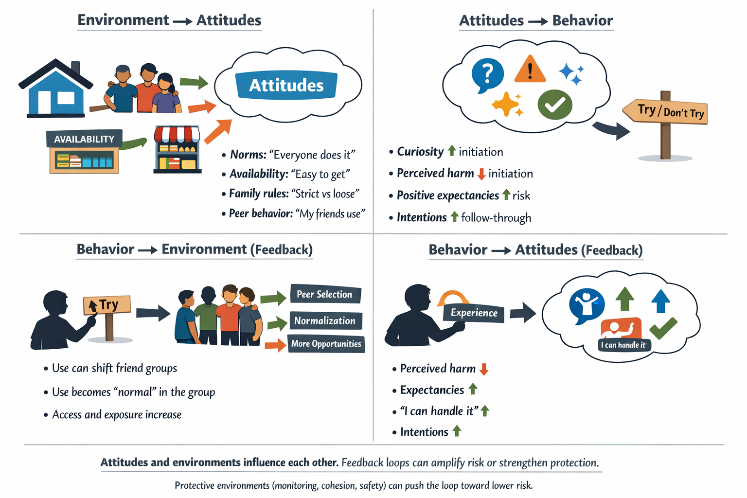
Attitudinal Predictors of Substance Use
Expectancies, Motives, and Curiosity
Positive beliefs about the effects of substances (e.g., “It will help me relax”) often predict experimentation. Curiosity, too, can double the likelihood of initiating use, making it a critical early-warning factor (Nodora et al., 2014). When adolescents hold high-risk cognitions—whether about perceived benefits or simply wanting to find out “what it’s like”—they are more prone to try substances (Pierce et al., 1996).
Intentions and Perceived Harm
An adolescent who already intends to use substances is likelier to follow through, especially in environments where use is normalized. Conversely, a strong perception of harm reduces the likelihood of initiation, demonstrating the power of accurate risk perceptions in prevention programs (Choi et al., 2002; Pierce et al., 1996).
Environmental Predictors of Substance Use
Parental and Family Environment
High parental monitoring—actively tracking a child’s whereabouts and social circle—consistently reduces early substance initiation (Buu et al., 2009). Strong family cohesion, open communication, and emotional warmth further protect against deviant behavior. Conversely, family conflict heightens the risk of early substance experimentation (Curran et al., 1997).
Neighborhood and Community Factors
Adolescents in unsafe or high-crime neighborhoods face additional stressors, increasing the likelihood of substance use as a coping mechanism (Buu et al., 2009). Easy access to drugs and alcohol in one’s community or social circle also amplifies initiation risk, reflecting how broader environmental contexts shape behavior.
Peer Attitudes and Influence
Youth are more likely to experiment with substances if their peers tolerate or engage in substance use (Curran et al., 1997). Moreover, those with lower resistance to peer pressure are particularly vulnerable (Dielman et al., 1990). Interventions that enhance adolescents’ ability to say “no” and reduce their exposure to deviant peer behaviors can help prevent initiation (Marshal et al., 2003).
Substance Availability
When substances are readily accessible—whether at home, in schools, or in the broader community—adolescents’ likelihood of using them increases. In families or communities aware of high substance availability, stricter rules and vigilant monitoring can mitigate some of this risk (Buu et al., 2009).
ABCD Substance Use Attitudes & Environments Survey Instruments
The ABCD Study assesses these attitudinal dimensions (e.g., expectancies, motives, perceived harm) and environmental contexts (e.g., home life, neighborhood and school, peers, and substance availabilities) through standardized tools (Lisdahl et al., 2018). See tables of these instruments in the Appendix to this chapter at the end of the document.
These multiple layers of influence—attitudinal, familial, and environmental—highlight why comprehensive data collection is crucial to understanding the many pathways of substance use. Before we can effectively analyze these complex predictors, however, the data itself must be prepared and validated through thorough cleaning processes.
Data Cleaning
The phrase “garbage in, garbage out” is often used to emphasize that the quality of the analysis depends on the quality of the data used. If the data is of poor quality, the results of the analysis will likely be flawed, regardless of the sophistication of the analysis techniques. Data cleaning is the process of ensuring the quality and integrity of the dataset, as issues like missing data, outliers, and inconsistencies can distort the results.
Data Quality
High-quality data should be accurate, complete, consistent, timely, and relevant to the analysis. Low-quality data can lead to incorrect conclusions and poor decision-making. Therefore, the first step in any data cleaning process is to assess the quality of the data.
- Accuracy: The data must correctly represent the real-world entities or conditions it is supposed to describe. For example, if a dataset records the ages of participants, the recorded ages should accurately reflect the participants’ actual ages.
- Completeness: The dataset should contain all necessary data points. Missing data can lead to biases and inaccuracies in the analysis. For example, if a dataset on youth substance use lacks data on key variables like age or gender, then conclusions drawn from the data may be unreliable.
- Consistency: The data should be uniform and not contradict itself. For example, imagine a dataset where one record shows that a participant reported “Never” using tobacco in a self-reported survey. However, in another part of the same dataset, the same participant is listed as having a nicotine metabolite present in their biological sample (which indicates recent tobacco use). This contradiction suggests an issue with the consistency of the data, as it presents conflicting information about the participant’s tobacco use. Such inconsistencies need to be identified and resolved during the data cleaning process to ensure accurate analysis.
- Timeliness: The data should be up-to-date and reflect the most current information available. Outdated data may not accurately reflect the current situation, leading to erroneous conclusions.
- Relevance: The data should be pertinent to the research question or hypothesis being tested. Irrelevant data can cloud the analysis and make it more difficult to draw meaningful conclusions.
Missing Data
What Are Missing Values?
Typically, the foremost problem in large-scale health research datasets is missing data. In data science, we often collect information to understand patterns, make predictions, or test hypotheses. However, sometimes pieces of this information are missing. A missing value occurs when no data is stored for a variable in an observation, often represented as blank cells, NULL, NaN, or NA. This can occur due to various reasons, such as participants skipping questions in surveys, data entry errors, or equipment malfunctions. In large, complex datasets like those used in health research, missing data is almost inevitable.
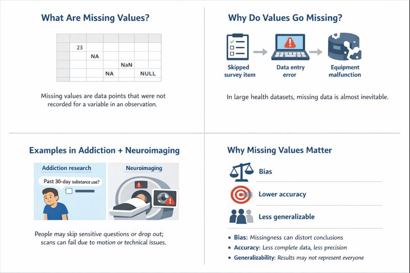
Why Do Missing Values Matter?
In addiction research, missing data is a common issue. For example, participants might skip questions about substance use due to embarrassment or fear of judgment, or individuals with severe addiction might drop out of studies, leaving gaps in the data. In neuroimaging studies, missing data can occur due to technical issues, such as equipment malfunctions or poor image quality can result in missing brain scans, or if a participant moves during scanning, the data may be unusable.
Missing values can create challenges in data analysis because many statistical methods require complete data. When values are missing, it can:
- Bias Results: Missing data can lead to incorrect conclusions if the missingness is related to what we are trying to measure.
- Reduce Accuracy: Analyses may be less precise because they are based on incomplete information.
- Affect Generalizability: Findings might not apply to the broader population if the missing data isn’t handled properly.
Types of Missing Data: MCAR, MAR, and MNAR
Not all missing data is the same. Understanding why data is missing helps researchers choose the best way to handle it. There are three main types of missing data mechanisms:
- Missing Completely at Random (MCAR)
- Missing at Random (MAR)
- Missing Not at Random (MNAR)
Definitions, Assumptions, and Examples
The table below summarizes each type, their definitions, assumptions, and provides examples from addiction research and neuroimaging studies.
| Type of missing data | Definition | Key assumption | Example in addiction research | Example in neuroimaging studies |
|---|---|---|---|---|
| MCAR (Missing Completely at Random) | The probability that a data point is missing is the same for all observations. Missingness is unrelated to observed or unobserved data. | Missing data form a random subset of the dataset with no systematic pattern. | A participant skips a survey question due to a random distraction (for example, a fire alarm), unrelated to their substance use or any measured variable. | A brain scan is missing because the MRI machine malfunctioned during the session, unrelated to the participant’s characteristics or behavior. |
| MAR (Missing at Random) | The probability that a data point is missing is related to observed data, but not to the missing value itself. | Missingness can be fully explained by other observed variables in the dataset. | Participants with higher observed stress levels are more likely to skip questions about substance use, but missingness is not related to their actual substance use (which is unobserved). | Imaging data are missing for participants who moved during the scan; movement is recorded and is related to observed anxiety levels during the session. |
| MNAR (Missing Not at Random) | The probability that a data point is missing is related to the missing value itself or to unobserved factors. | Missingness depends on unmeasured variables or the value of the missing data, even after accounting for observed data. | Participants with more severe substance use choose not to report their use due to stigma, so missingness is directly related to the level of substance use. | Participants with certain unobserved brain abnormalities produce unusable scans because their condition affects the imaging process, making missingness related to unmeasured brain characteristics. |
Data Inspection
To identify missing values, as well as other aspects of datasets for cleaning, we must identify the issues. This step involves thoroughly reviewing the dataset to detect inconsistencies, missing values, outliers (data points that have extreme values), or any other irregularities. The goal of data inspection is to understand the nature of the data and identify areas that require cleaning.
Data inspection includes:
- Visual Inspection: Using visualizations such as histograms, box plots, or scatter plots helps spot outliers or unusual patterns in the data. These visual tools provide a quick overview of the data’s distribution and highlight areas that may require attention.
- Summary Statistics: Calculating summary statistics like mean, median, mode, standard deviation, and range gives insight into the data’s central tendency and variability. This can help identify anomalies such as outliers or unexpected values.
- Checking for Duplicates: Duplicate entries can skew the results of an analysis by giving undue weight to certain data points. Identifying and removing duplicates ensures that each data point is only represented once in the analysis.
- Data Profiling: Data profiling involves analyzing the dataset’s structure, distribution, and relationships between variables. Tools like Pandas in Python can generate comprehensive reports on the data, highlighting potential issues that may need to be addressed during the cleaning process.
Many of these methods for data inspections were previously covered in Modules 2 and 3 on univariate and bivariate exploratory data analysis.
Handling Missing Data
After identifying missing values in the inspection steps, researchers must properly address the missing data to ensure the validity and reliability of research findings. Best practices involve using advanced statistical methods that make the most of the available data while minimizing bias. The first common advanced methods Maximum Likelihood Estimation (MLE), which is a statistical method that estimates the missing values based on patterns within existing data. The second, Multiple Imputation, is a method where each missing value is replaced with a set of plausible values that represent the uncertainty about the right value to impute. These multiple datasets are then analyzed separately, and the results are combined to produce estimates that reflect the missing data’s uncertainty.
Ad Hoc Methods
While advanced methods are preferred, sometimes simpler, ad hoc methods are used in specific situations. These methods are easier to implement but come with trade-offs in terms of bias and statistical validity. Appendix includes Table 3.4 which summarizes basic ad hoc methods for handling missing data, along with their descriptions, advantages, and disadvantages, adopted from van Buuren (2018).
Choosing the Right Method
Selecting the appropriate method to handle missing data depends on:
- Understanding whether data is MCAR, MAR, or MNAR guides the choice of method.
- With minimal missingness, simpler methods may suffice.
- Advanced methods reduce bias but are more complex to implement.
Addressing Outliers
Beyond missing values, data cleaning may also involve addressing outliers that can bias findings. Outliers are data points that differ significantly from other observations in a dataset.
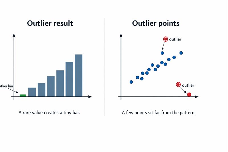
Outliers should be dealt with carefully because they can either represent valuable insights or introduce bias into the analysis.
- Examination: Outliers should be reviewed to determine whether they are genuine data points or the result of errors. Genuine outliers may provide valuable insights, while erroneous outliers should be corrected or removed. This step is crucial in addiction research, where extreme values might reflect significant cases important for understanding substance use patterns.
- Capping: Capping involves limiting outliers to a certain percentile (e.g., the 1st and 99th percentiles) to reduce their impact on the analysis. For example, in a dataset of alcohol consumption, capping might involve setting a maximum threshold that aligns with the majority of the data, ensuring that extreme cases do not skew the analysis.
- Transformation: Applying mathematical transformations, such as logarithmic or square root transformations, can minimize the impact of outliers and make the data more suitable for analysis.
In addiction research, outliers can be particularly important data points and often should not be ignored or excluded. For example, in neuroimaging studies of individuals with substance use disorders, an outlier might be a brain scan showing significantly higher or lower activity in a particular region associated with reward processing. This could represent a unique neural adaptation or an extreme addiction case that offers insights into the neurological impacts of prolonged substance use. Therefore, researchers must plan for handling outliers thoughtfully, considering the context of the data and the potential implications for their findings.
Correcting Inconsistencies
Inconsistencies in data refer to variations or discrepancies within the dataset that can lead to inaccurate analyses or conclusions. These inconsistencies might include differences in formatting, units of measurement, or duplicate entries that can distort the findings if not addressed properly.
- Standardizing Formats: Data entries should follow a consistent format across the dataset. For example, dates should be in the same format (e.g., YYYY-MM-DD) throughout the dataset. Consistency in formatting ensures that all data points are comparable and can be analyzed accurately without introducing errors due to format differences.
- Normalization: Normalization involves scaling data to bring all values into a similar range or scale. This is especially important when dealing with variables measured on different scales. For instance, substance use frequency might be measured on a scale of 1 to 10, while neuroimaging data might be recorded in millimeters of brain activity. Normalizing these variables ensures that they can be compared and analyzed together without any one variable disproportionately influencing the results.
- Dealing with Duplicates: Duplicate records should be removed or consolidated to prevent them from distorting the analysis. In some cases, duplicates may need to be investigated to determine whether they represent genuine repeated measurements or erroneous entries.
In addiction research, correcting inconsistencies is particularly important because inconsistent data can lead to misleading conclusions. For example, in a study examining the effects of substance use on brain structure, inconsistent labeling of brain regions across different scans could result in inaccurate interpretations of how substance use impacts specific brain areas. Addressing such inconsistencies is essential for ensuring that the findings are valid and can be reliably reproduced in future research.
Verifying the Cleaning
After the data has been cleaned, researchers need to verify that the cleaning process was successful and that no new errors were introduced. This step ensures that the dataset is now accurate and ready for analysis. This is typically done by performing a second round of data inspection, using the same techniques as in the initial inspection, to confirm that issues have been resolved. This step helps ensure that the cleaning process did not introduce new errors or inconsistencies. In some cases, researchers can use cross-validation by comparing the cleaned dataset against known values or a separate, clean dataset can help verify accuracy. This step is especially important when dealing with complex datasets or when the cleaning process involved significant changes.
Reporting the Cleaning
Reporting the data cleaning process is essential for transparency, reproducibility, and ensuring that the analysis is understood in context. This includes documenting any changes made to the dataset, the rationale behind those changes, and how those changes might impact the analysis. Key elements to include in the report:
- Overview of Issues Identified: Summarize the main issues found during the initial data inspection. This provides context for the cleaning process and helps others understand the challenges faced.
- Cleaning Methods Used: Detail the specific methods and tools used to clean the data, including how missing data, outliers, and duplicates were handled. This information is crucial for replicating the analysis or understanding how the data was prepared.
- Impact on the Analysis: Discuss how the cleaning process might affect the results of the analysis and any limitations that the cleaned data may still have. This section should also address any potential biases or errors that remain in the dataset.
Role of Data Structure and Curation in Data Cleaning
A well-defined data structure and rigorous data curation process in the ABCD Study greatly streamline the subsequent data cleaning and decision-making. Data structure refers to how the ABCD data are organized and formatted. ABCD data are released through the NIMH Data Archive (NDA) in structured tables (NDA “data structures”), each typically corresponding to a specific assessment or measure (NIMH, n.d.). Every such data structure includes standardized key fields – for example, each table contains the participant’s global unique identifier (GUID), age (in months), sex, date of assessment, and the study-specific subject ID. Related variables from an instrument are grouped together in one place, and all records share common identifiers and time stamps. This consistency makes it easier to merge datasets, track each participant across different measures, and spot irregularities. If an outlier or inconsistency appears in one variable, the structured format allows analysts to quickly cross-check it against other variables from the same assessment or time point.
Data curation involves applying standards and quality checks to the dataset before public release, ensuring that the data adhere to uniform conventions. The ABCD curators follow NDA harmonization standards so that variables are consistently defined across the study. In practice, the NDA curation team “maps identical Data Elements across Data Structures” so that the same data item (e.g. a questionnaire question asked at multiple waves or a common demographic variable) uses the same name, format, and coding wherever it appears (NIMH, n.d.). This harmonization means researchers don’t have to reconcile different coding schemes for the same construct – the curation process has already aligned them. For example, if a yes/no question appears in several instruments, the curated data will use one standardized coding for “Yes” and “No” in all instances. Researchers can thus apply cleaning operations (like recoding or factorizing a categorical variable) once and trust that it applies uniformly across the dataset.
ABCD data curation standards also enforce codes and documentation for missing or special values, which directly facilitates cleaning decisions (ABCD Study, .n.d.). The ABCD data use standardized missing value codes to indicate why data might be absent or not applicable. For instance, a response of 777 generally means the participant “declined to answer,” and 999 means “don’t know,” as consistent codes across the database. Additionally, many ABCD measures implement skip logic (gating), so certain questions are only asked when applicable; unanswered fields can thus be distinguished as deliberate “not applicable” skips rather than true random missingness.
These structured codes and skips preserved in the curated data allow analysts to distinguish different types of missing data – e.g. refusals vs. logical skips vs. accidental omissions – at a glance. Crucially, the reason behind a missing value is recorded in the data itself, “allowing analysts to distinguish between refusals, uncertainty and random omissions when deciding how to handle missing data”. This clarity guides the cleaning process: one would likely treat a 777 (“refused”) differently from a blank that indicates a skipped question. It also helps analysts assess the missingness mechanism (MCAR, MAR, or MNAR) because the presence of structured skip patterns and non-response codes makes the origin of missingness explicit. If many values are 777 (refusal), those missing data are Not at Random by nature and might warrant a different imputation strategy (or even exclusion) compared to data that are missing completely at random. By having these curation standards in place, researchers can apply appropriate missing-data handling techniques with greater confidence, knowing the context for each missing value.
In summary, the data structure and curation standards in ABCD ensure that the dataset arrives to analysts in a clean, consistent form that requires minimal heavy lifting. Much like upfront quality control during data collection, a robust data structure and thorough curation preemptively resolve many issues that would otherwise complicate cleaning. Each ABCD data release is a curated dataset in which gross errors, out-of-range values, and inconsistent coding have been addressed or flagged according to documented standards. This leaves the researcher with data that are more interpretable and uniform, so the role of cleaning shifts from hunting for errors to fine-tuning for analysis. In effect, better-organized and curated data make the cleaning stage “less about ‘garbage removal’ and more about fine-tuning,” supporting more reliable and transparent research outcomes.
Works Cited
ABCD Study. (n.d.). Curation standards. National Institutes of Health. https://docs.abcdstudy.org/latest/documentation/
Alexander, B. (1973). Human behavior and the social environment: Selected papers from the Rat Park series. Canadian Journal of Behavioural Science, 5(3), 271–283.
Arthur, M. W., Hawkins, J. D., Pollard, R., Catalano, R. F., & Abbott, R. D. (2007). Measuring risk and protection in communities using the Communities That Care Youth Survey. Evaluation and Program Planning, 30(3), 197–211. https://doi.org/10.1016/j.evalprogplan.2007.07.002
Bartels, D., Jupp, D., & Wit, H. (2016). Substance use exposure in households: Storage and access patterns among youth. Journal of Substance Abuse Treatment, 58, 10–19. https://doi.org/10.1016/j.jsat.2016.04.004
Bingham, C. R., et al. (1995). Peer behavior profile: Assessment of youth peer influences. Journal of Youth and Adolescence, 24(2), 213–227. https://doi.org/10.1007/BF02286454
Buu, A., McCartan, C., Lamb, K., Benning, K., Schmidt, D., & Rothman, E. (2009). Parent, family, and neighborhood effects on the development of child substance use and other psychopathology from preschool to the start of adulthood. Journal of Studies on Alcohol and Drugs, 70(4), 489–498. https://doi.org/10.15288/jsad.2009.70.489
Choi, W. S., Gilpin, E. A., Farkas, A. J., & Pierce, J. P. (2002). Determining the probability of future smoking among adolescents. Addiction, 96(4), 313–323. https://doi.org/10.1046/j.1360-0443.2002.00305.x
Curran, C. P., & Marczinski, C. A. (2017). Taurine, caffeine, and energy drinks: Reviewing the risks to the adolescent brain. Birth Defects Research Part C: Embryo Today: Reviews, 109(6), 1640–1648. https://doi.org/10.1002/bdr2.1054
Curran, P. J., Stice, E., & Chassin, L. (1997). The relation between adolescent alcohol use and peer alcohol use: A longitudinal random coefficients model. Journal of Consulting and Clinical Psychology, 65(2), 130–140. https://doi.org/10.1037/0022-006X.65.2.130
Dielman, T. E., Butchart, A. T., & Shope, J. T. (1990). Structural equation model tests of patterns of family interaction, peer alcohol use, and intrapersonal predictors of adolescent alcohol use and misuse. Journal of Drug Education, 23(3), 273–316. https://doi.org/10.2190/9F1C-T4X7-9VK6-25F9
Dishion, T. J., & Kavanagh, K. (2003). Intervening in adolescent problem behavior: A family-centered approach. Guilford Press.
Dishion, T. J., Nelson, S. E., & Kavanagh, K. (2003). The Family Check-Up with high-risk young adolescents: Preventing early-onset substance use by parent monitoring. Behavior Therapy, 34(4), 553–571. https://doi.org/10.1016/S0005-7894(03)80019-6
Karoly, P., Dishion, T., & Leve, L. (2016). Adolescent monitoring and risk for substance use: A longitudinal analysis. Journal of Child Psychology and Psychiatry, 57(3), 313–323. https://doi.org/10.1111/jcpp.12428
Karoly, P., Dishion, T., Leve, L., & Tieman, B. (2015). Parental monitoring and adolescent substance use: The role of family dynamics and peer influence. Journal of Family Psychology, 29(5), 701–712. https://doi.org/10.1037/a0039032
Lisdahl, K. M., Sher, K. J., Conway, K. P., Gonzalez, R., Feldstein Ewing, S. W., Nixon, S. J., Tapert, S., Bartsch, H., Goldstein, R. Z., & Heitzeg, M. (2018). Adolescent brain cognitive development (ABCD) study: Overview of substance use assessment methods. Developmental Cognitive Neuroscience, 32, 80–96. https://doi.org/10.1016/j.dcn.2018.02.007
Marshal, M. P., Molina, B. S., & Pelham Jr, W. E. (2003). Childhood ADHD and adolescent substance use: An examination of deviant peer group affiliation as a risk factor. Psychology of Addictive Behaviors, 17(3), 293–302. https://doi.org/10.1037/0893-164X.17.3.293
Moos, R. H., & Moos, B. S. (1994). Family environment scale manual (3rd ed.). Consulting Psychologists Press.
Mujahid, M. S., Diez Roux, A. V., Marceau, K., Sheppard, L., Kawachi, I., & Cubbin, C. (2007). Neighborhood safety and depressive symptoms in older adults: The role of physical activity and social cohesion. Social Science & Medicine, 65(7), 1573–1586. https://doi.org/10.1016/j.socscimed.2007.03.024
National Institute of Mental Health. (n.d.). Guidance for preparing REDCap data for NIMH Data Archive submission. National Institutes of Health. https://s3.amazonaws.com/nda.nih.gov/Documents/Guidance+for+Preparing+REDCap+Data+for+NDA.pdf
Nodora, J., et al. (2014). Curiosity as a predictor of smoking experimentation independent of susceptibility in a US national sample. Addictive Behaviors, 39, 1695–1700. https://doi.org/10.1016/j.addbeh.2014.07.009
Sobell, L. C., & Sobell, M. B. (1992). Timeline followback: A technique for assessing self-reported ethanol consumption. In R. Litten & J. Allen (Eds.), Measuring alcohol consumption: Psychosocial and biochemical methods (pp. 41–72). Humana Press.
Steinberg, L., & Monahan, K. C. (2007). Age differences in resistance to peer influence. Developmental Psychology, 43(6), 1531–1543. https://doi.org/10.1037/0012-1649.43.6.1531
van Buuren, S. (2018). Flexible imputation of missing data. Chapman & Hall/CRC Interdisciplinary Statistics Series.
Appendix
ABCD Substance Use Attitudes and Environmental Survey Instruments
For more information on the instruments, see the substance use domain in the ABCD wiki: https://wiki.abcdstudy.org/release-notes/non-imaging/substance-use.html
| Instrument Name | Years & Table (5.0) | Instrument Description |
| Alcohol Expectancies – Brief Adolescent (AEQ-AB) | Baseline to 3-Year, 5-Year, 7-Year (su_y_alc_exp) | Measures thoughts, feelings, and beliefs about alcohol’s effects. Used to assess alcohol expectancy effects. |
| Alcohol Motives (PhenX) | 4-Year Follow-Up, 6-Year Follow-Up (su_y_alc_motiv) | Assesses coping and enhancement motives for drinking alcohol using a 20-item scale. |
| Marijuana Expectancies (MEEQ-B) | Baseline to 3-Year, 5-Year, 7-Year (su_y_can_exp) | Measures beliefs about marijuana’s effects. |
| Marijuana Motives (PhenX) | 4-Year Follow-Up (su_y_can_motiv) | Assesses coping and enhancement motives for marijuana use with a 25-item scale. |
| Vaping Expectancies | 3-Year, 5-Year Follow-Up (su_y_vap_exp) | Measures beliefs about vaping’s effects. Adapted from the Marijuana Expectancies measure. |
| Vaping Motives | 2-Year, 4-Year Follow-Up (su_y_vap_motiv) | Assesses reasons for vaping, developed by the ABCD Substance Use workgroup. |
| Cigarette Expectancies (ASCQ) | Baseline to 3-Year, 5-Year, 7-Year (su_y_nic_exp) | Measures beliefs about the effects of smoking nicotine. |
| Tobacco Motives | 4-Year, 6-Year Follow-Up (su_y_nic_motiv) | Assesses motives for using tobacco products. |
| ENDS Expectancies (CEQ) | 3-Year, 5-Year, 7-Year (su_y_ends_exp) | Measures beliefs about using electronic nicotine delivery systems (ENDS). |
| ENDS Motives | 4-Year, 6-Year Follow-Up (su_y_ends_motiv) | Assesses motives for using ENDS. |
| Reasons for ENDS Use | 4-Year, 6-Year Follow-Up (su_y_ends_reas) | Assesses reasons for using electronic nicotine delivery systems (ENDS). |
| PATH Intention to Use | Baseline to 4-Year Follow-Up (su_y_path_intuse) | Measures youth’s intentions to use alcohol, nicotine, and marijuana. |
| Perceived Harm SU (PhenX) | Baseline to 4-Year Follow-Up (su_y_percharm) | Assesses youth’s beliefs about the risks associated with substance use. |
| Instrument Name | Years of Administration & Table Name (5.0) | Instrument Description |
| Parental Monitoring | Annually since baseline | ce_y_pm | Assesses a parent’s active efforts to track a child’s whereabouts and activities. Derived from previous measures (Karoly et al., 2016; Stattin & Kerr, 2000). |
| Family Environment Scale (PhenX) | Annually since baseline | ce_y_fes | Measures family conflict and cohesion, assessing the emotional climate and support among family members (Moos & Moos, 1994). |
| Peer Behavior Profile | Annually since 2-year follow-up | ce_y_pbp | Evaluates youth friendships with prosocial or rule-breaking peers. The two subscales assess how the youth’s network influences their behavior (Bingham et al., 1995). |
| Peer Network Health: Protective Scale | Annually since baseline | ce_y_pnh | Assesses protective peer behaviors that reduce the likelihood of engaging in risky actions like substance use. |
| Resistance to Peer Influence | 4-year follow-up | ce_y_rpi | Assesses youth’s ability to resist peer pressure and maintain independent decision-making (Steinberg & Monahan, 2007). |
| School Risk and Protective Factors (PhenX) | Annually since baseline | ce_y_srpf | Measures school climate and youth engagement in school using three subscales: School Environment, School Involvement, and School Disengagement. Based on Communities That Care Survey (Arthur et al., 2007). |
| Neighborhood Safety/Crime Survey (PhenX) | Baseline; 1-, 2-, and 4-year follow-up | ce_y_nsc | Assesses youth perceptions of neighborhood crime and safety using a 5-point Likert scale. Adapted from the PhenX Neighborhood Safety Protocol (Mujahid et al., 2007). |
| Community Risk and Protective Factors (Youth) | Annually since 2-year follow-up | su_y_crpf | Measures youth perceptions of risk and protective factors in their community, particularly access to substances. |
| Sibling Use | Annually since 3-year follow-up | su_y_sibuse | Assesses the use of alcohol, cannabis, tobacco, and other substances by siblings and its influence on youth. |
| Method | Description | Advantages | Disadvantages |
|---|---|---|---|
| Listwise Deletion | Removes any case (row) that has one or more missing values for the variables being analyzed. | – Simple to implement – Results are unbiased if data are MCAR |
– Can significantly reduce sample size – Potentially biased if data are not MCAR – Loss of information |
| Pairwise Deletion | Uses all available data to calculate statistics, considering all cases where the pair of variables is present. | – Utilizes more data than listwise deletion | – Can produce inconsistent results – Correlation matrix may not be positive definite – Assumes MCAR |
| Mean/Mode Imputation | Replaces missing values with the mean (for continuous variables) or mode (for categorical variables) of the observed data. | – Easy to implement – Preserves sample size |
– Underestimates variability – Biases estimates towards the mean – Can distort relationships between variables |
| Regression Imputation | Predicts missing values using a regression model based on other observed variables. | – Accounts for relationships between variables | – Underestimates variability – Can overfit data – Assumes linear relationships – Can bias correlations upwards |
| Stochastic Regression Imputation | Similar to regression imputation but adds random error to the predicted values to reflect uncertainty. | – Preserves variability better than regression imputation | – More complex – Randomness can introduce noise – Still assumes correct model specification and MAR |
| Last Observation Carried Forward (LOCF) | For longitudinal data, replaces missing values with the last observed value for that individual. | – Simple – Maintains within-subject data structure |
– Can introduce bias – Assumes no change over time – Not suitable for all types of data |
| Indicator Method | Creates a binary indicator variable for missingness and includes it in the analysis model. | – Retains all cases – Accounts for missingness pattern |
– Can lead to biased parameter estimates – Assumes missingness is informative – May not correct bias in estimates |
