7 Habitat Assessment
The first chapter in the habitat-focused techniques group centers on the idea of habitat assessment. Many land use management plans have been based on habitat analyses to explore different future scenarios. In recent years, computing developments have enabled the emergence of landscape scale habitat modeling to explore complex options for ecosystem management. This chapter will present principles of habitat analysis and landscape scale modeling methods, which are often linked with habitat suitability for specific species, and how these ideas are used in practice to mitigate habitat losses and evaluate tradeoffs. We will end with a case study on habitat assessment in the Florida Everglades.
HISTORY AND PURPOSE OF HABITAT ASSESSMENT
Natural resource management has traditionally focused on populations. Starting in the 1970s and 1980s, natural resource management agencies increasingly employed habitat-based approaches for resource inventory and assessment (Bain and Stevenson 1999). Now, habitat is the common basis of most impact assessments, resource inventories, species management plans, and mitigation planning. Animal and plant populations fluctuate through time while habitat is much more stable. Habitat can be defined in clear and intuitive physical terms by linking habitat with specific species’ known tolerances and needs. Also, the quality of a habitat can be related to species preferences. Thus, habitat is a tangible resource that can be measured and modeled for considering future scenarios of change. This resource can be quantified and used in negotiations and decision-making about development proposals. It can also be included in mitigation strategies when compensating for habitat losses. For these practical reasons, natural resource management agencies have turned to habitat as the basis for negotiating proposed developments and environmental changes.
Habitat assessment has been built into the United States’ environmental laws to enhance the practicality and effectiveness of species conservation. Under the National Environmental Policy Act (NEPA), habitat is frequently assessed and is the common basis for evaluating mitigation measures for habitat loss. The Endangered Species Act (ESA) also requires protection of habitat for endangered species. Finally, the Fish and Wildlife Coordination Act (FWCA) requires that federal agencies analyze potential impacts to habitat, consider habitat when evaluating development options, and mitigate habitat losses. This Act most often engages the United States Fish and Wildlife Service (USFWS) in species conservation and requires it to consult with other federal agencies that issue permits, manage landscapes, or administer federal projects. Agencies at the state level and/or the National Marine Fisheries Service (NMFS) can also become involved. Thus, taking habitat into account is not only practical and necessary when considering environmental impacts, but its assessment is often required by some United States environmental laws.
Habitat assessment started due to the need to account for habitat losses from development and federal projects, like dams. Computer technology and geographic information systems (GIS) have expanded the use of habitat data and modeling to predict species ranges, analyze landscape transformation, and predict ecosystem change (Gurnell et al. 2002). Regional conservation planning has also extended the role of habitat to address biodiversity by seeking habitats supporting multiple conservation-priority species. Habitat fundamentals remain intact, but the expansion of habitat to the regional, state and ecosystem scales brings new opportunities for its use.
Methods for habitat assessments and modeling are important tools for many agencies and organizations with a mission for environmental conservation and management. Habitat assessments are influential in protecting some areas against forest harvesting, development, and new detrimental land uses. When habitats are quantified and found to be of high-use for valued or protected species, this information can shape other land management decisions. Also, assessment of habitat status is commonly used to set animal stocking levels, plan restorations, and determine the need for rehabilitation. Limitations on species abundance and poor habitat properties can guide habitat improvements. Predicting species distribution or estimating the suitability of habitat for a species contributes to the justification for management attention. Some state natural resource management agencies and conservation groups use this large scale information to plan land acquisitions and land-management objectives. Linking habitat models with data in a GIS is very valuable in identifying lands and waters that merit consideration for species protection. Maps of key habitats for endangered species or species popular in the public arena can inform regulatory decisions like the placement of pipelines, roads, and other relocatable infrastructure. Finally, habitat assessment results and habitat maps are often used by managers to determine specific needs, and make presentations to the public, agencies, conservation organizations, and legislators. All these uses of habitat assessments and their resulting data are now routinely incorprated into agency and organizational conservation activities.
THEORETICAL BASIS FOR HABITAT ASSESSMENT
Defining the physical conditions and limiting factors that quantify the habitat requirements for a species has a long history in ecology (Pianka 1966; Rosenzweig 1981). Habitat is tied in with the concept of a niche (Pulliam 2000; Hirzel and Le Lay 2008). Specifying a niche is equivalent to defining habitat conditions that allow a species to persist in space and time. When the habitat for a species is specified, it can be used to predict potential presence and absence. When habitat conditions are rated for quality, then predictions of species abundance can also be made. In the last century, science has made important contributions to the conservation and management of many species by defining their habitat needs (Southwood 1977). All this information regarding habitats was gathered by observing species in their natural settings and documenting the habitat conditions where they lived. This field of study was often referred to as natural history.
The term niche was given different meanings early in the 1900s. The original definition focused on the environmental requirements for a species (Grinnell 1917). Elton (1927) used a different definition of the niche, which characterized the role of a species in a community. Habitat is more consistent with the first definition of the niche, and Hutchinson (1957) elaborated on this definition. The fundamental niche is an n-dimensional hypervolume that is consistent with a range of habitat parameters. You can visualize this concept by thinking about several distinct habitat dimensions, like temperature, elevation, soil moisture, and others, that encompass the conditions needed for a species’ survival. The fundamental niche often will not be fully occupied. The realized niche is the smaller portion that is occupied by a species, and is shaped by interaction with other species and limiting resources. Thus, investigations to define habitat using the niche theory most often seek to identify key variables, responses by a species to variation in variables, and the interactions among variables. The realized niche that often defines habitat is based on occupied space.
HABITAT SUITABILITY CONCEPTS
Species distribution models are based on environmental conditions in occupied habitats. Sometimes called habitat suitability maps, these models combine data on species presence or abundances with data from measurements of key habitat variables (example in Figure 7.1). Then a statistical model is used to relate the two data sets to define both tolerable habitat conditions and optimal habitats with high densities of individuals. The fundamental assumption is that individuals will select habitats most suitable to their survival. As more individuals select these habitats, the benefits of new individuals will decline because of intra-specific competition (crowding). This pattern of high abundances in the best habitats is to be expected since these habitats can support the most individuals. This pattern is termed the ideal free distribution (Fretwell and Lucas 1970, Fretwell 1972), which supports the link between high density of a species in a habitat with high suitability (Fraser and Sise 1980). Data on these high suitability habitats are collected by field measurements, meterological stations, digitized maps, aerial photographs, and satellite images. Once species presence and density data are combined with habitat data, a definition of niche and habitat requirements can be specified. These results can then be used in a GIS for predicting spatial distributions of species (Beutel et al. 1999; Guisan and Zimmermann 2000; Anderson et al. 2003; Rushton et al. 2004; Guisan and Thuiller 2005; Hirzel et al. 2006). Other analyses can be performed for assessing ecological impacts of habitat change and the effects of climate change on species distributions.
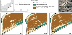
Research has shown that there can be errors in the basic study design linking presence and abundance to physical habitat conditions (Fielding and Bell 1997). Data are often collected within a narrow time frame, which can lead to bias when defining a habitat due to higher or lower population levels, climatic conditions, and resource availability levels. Competitors and predators can restrict a species’ use of suitable habitat, leading it to abandon what would normally be considered suitable habitat conditions. There are questions about which spatial scale is more appropriate to use when quantifying habitats (Turner et al. 1989; knight and Morris 1996; Gustafson 1998). Often, the presence of a single individual is not necessarily a clear indicator for determining the area in which the individual may normally respond to habitat conditions. This varies by species and researchers often go by whatever works best when performing habitat data collection in the field. For species that are more flexible in their use of habitat, or generalists, it is often difficult to identify preferences for specific habitat conditions, or the physical parameters that may influence habitat use or position. By contrast, the conditions that are critical to the survival of a species with specialized habitat conditions, such as birds that nest in grasslands, are more easily identifiable. Finally, it is not always clear which physical variables may need to be accounted for when defining a habitat and assessing its suitability. Investigators often collect data on multiple habitat properties, but it is possible that some key properties might be missed.
There is a second dimension of uncertainty about linking species and habitats. False absences can occur even when suitable habitat is present because other factors may be preventing a species from occupying the area. Absence in suitable habitats can come from localized elimination of a species by things like harvest or disease, restricted dispersal by barriers, habitat that is too small to support a population, and biotic interactions that drive individuals out of their preferred habitats (Meixler 2021). These phenomena can skew the definition of suitable habitat in inaccurate ways. Likewise, false presences, or presence in unsuitable habitats, can also occur (Meixler et al. 2009). Crowding may induce individuals to inhabit fringe locations, and sub-dominant individuals can be displaced to marginal or unsuitable habitats. Movement across unsuitable habitats during migration can also happen. Also, territorial behavior can force some individuals out of highly suitable habitats. And, habitat generalists often follow their food source which can cause them to switch between habitats constantly. Finally, false presences in marginal or unsuitable habitats can alter the definition of suitable habitat and broaden the range of habitat properties considered.
HABITAT SUITABILITY MAPPING AND MODELING
Habitat quantification is vital to mapping species distribution for research on biogeography, ecology, changing climate impacts, invasive species ranges, and other investigations (Franklin 2010). Generally, species distribution maps use the fundamental niche and the widest range of suitable conditions for many detailed studies. Habitat definitions are combined with commonly available spatial data like topography, soils, climate, and vegetation maps, in a GIS to produce species distribution maps. This is a relatively novel use of habitat definitions due to the increased availability of spatial data, GIS integration of data, and mapping capability (Brooks 1997). Often, many species are mapped in this way to identify areas of high biodiversity for conservation strategy development.
The dominant demand for estimating habitat suitability was to perform impact assessments for key species. Quantification of habitat for proposed developments and mitigation needs drove applied habitat modeling. In the 1980s, the USFWS developed standardized Habitat Evaluation Procedures (HEP) to use in impact assessments, which is part of the agency’s mandate (United States Fish and Wildlife Service 1980a, United States Fish and Wildlife Service 1980b). Professional judgment and ad hoc methods were not persuasive enough to be effective in modifying the plans of other agencies, large scale developments, or for specifying mitigation measures for losses of habitat. The USFWS adopted HEP to meet several critical objectives of impact assessment. These objectives included: 1) Displaying data on present conditions and proposed development options, 2) Predicting fish and wildlife habitat changes over time with proposed changes, 3) Ensuring a method that is practical to implement using commonly available data, readily available for species habitat models, and cost effective to execute, and 4) Making sure the method is sensitive to habitat losses and the magnitudes of changes in habitat quality. The HEP fills this need and is composed of: 1) Habitat Suitability Index (HSI) models to assess habitat quality for many species, and 2) Accounting procedures to predict the impacts of proposed developments. HSI models are used to infer the ability of a habitat to support a species and are thus positively correlated with carrying capacity (Schamberger and Krohn 1982; Dussault et al. 2006). HSI models produce an index between 0 and 1, with 0 designating unsuitable habitat and 1 being optimal habitat. The HSI is calculated as study area/optimal habitat conditions, where conditions are represented by variables that include: 1) Whether the species responds; 2) If it can be readily measured; 3) If it can be predicted in the future under change; or 4) if it is influenced by projects or management (Schamberger and O’Neil 1986). The USFWS created a library of hundreds of HSI models for indicator species and other valued species (United States Fish and Wildlife Service 1981). To implement HSI models confidently, they must be tested for accuracy (i.e., validated). Validation involves testing the performance of an HSI model against independent quantitative data in space and time, such as against population density or abundance (Zorn et al. 2011; Zajac et al. 2015; Theuerkauf and Lipcius 2016).
HEP is based on combining a measure of habitat quantity (e.g., affected habitat area, in acres or hectares) with an index of habitat quality (e.g., HSI, 0 to 1 scale) to determine habitat units (dimensionless numbers) (United States Fish and Wildlife Service 1980b). The relationship is expressed as:
Habitat area x Habitat quality (HSI) = Habitat units (HUs)

The HEP have been in common use to estimate impacts to fish and wildlife species, compare development options, and set mitigation requirements (Urich and Graham 1983). Figure 7.2 shows an example in which the change in wetland habitat units are shown over time with and without a railroad construction project. The HEP are not meant to be research tools, carrying capacity estimators, population models, or be comprehensive.
The USFWS developed a similar set of procedures for predicting habitat units in rivers and streams un- der different flow levels. The instream flow incremental methodology (IFIM; Stalnaker et al. 1995) was comprised of a habitat simulator for a river reach (Physical HABitat SIMulation, PHABSIM) which could be used to depict the amount and quality of habitat at different flow levels (Milhous et al. 1984). The changing spatial distributions of physical attributes of a river (e.g., water depth, current velocity, and substrate) as a result of variations in flow and the biological responses of aquatic species to these changes, provide the basis for simulating the consequences of ecosystem alteration. USFWS produced a library of suitability plots for each life stage of many valued fishes and other aquatic species. The weighted usable areas formed the basis for comparison of different flows by season, which could then be used for predicting the habitat conditions that might exist over the course of a species’ life history, since different life stages of a species require different habitat conditions. The charts, depicting flow rates and usable area for a species by season, defined the basis for negotiations on how much water was needed per season.
EXAMPLE APPLICATION OF HEP
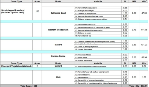
A HEP Assessment was performed on a land parcel in the Yakama Nation (Table 7.1) (Ashley and Muse 2008). A baseline HEP analysis was conducted on the Carl property (160 acres) in June 2007 to determine the number of habitat units to credit Bonneville Power Administration (BPA) for providing funds to acquire the property as partial mitigation for habitat losses associated with construction of the McNary Dam. The types of landcover present at that time were shrub/grassland (covering 99% of the area) and emergent wetland (covering 1% of the area). HEP model selection was based on the habitat types present and the species models identified in the McNary Dam Loss Assessment. The chosen species included: California quail (Callipepla californica), western meadowlark (Sturnella neglecta), mallard (Anas platyrhynchos), Canada goose (Branta canadensis), downy woodpecker (Dryobates pubescens), yellow warbler (Setophaga petechia), spotted sandpiper (Actitis macularius), and mink (Mustela vison). Sampling transects were utilized to collect field data for use in the models. The results provided information on habitat suitability (HSI) and habitat units for the land cover types in which each species resided (Ashley and Muse 2008).
Table 7.1: HSI and HU summary for Yakama Nation HEP project. Source: Ashley and Muse 2008
LIMITATIONS OF HABITAT SUITABILITY MAPPING
The application of habitat models and assessments can be unclear for cases that are controversial for regulatory and planning purposes. The real definition of habitat is dictated by the specific needs of a species, which has physical requirements for occupancy, survival, and reproduction. At the species level, habitat can be bounded and assigned a quality value using information about the species ‘ particular needs. Often classes of habitats are loosely discussed, like old growth forests, riparian zones, and grasslands, whose characteristics might be decoupled from those of the precise species under consideration (Hall et al. 1997). This approach often implies that a habitat can house a collection of species, but that is confusing and imprecise in its definition. Habitat quality should refer to the optimal physical conditions for species survival and population persistence. Habitat models often define physical conditions as high-quality habitat based on the preferred conditions of a species. These high quality habitats are considered to accommodate high densities of a particular species. Considering habitat in such a loose manner introduces ambiguity into the definitions and quality assessments of habitats, which makes it hard to pinpoint the precise effects of any given proposal. Applications of the term habitat should be based on a species-specific foundation, and backed up with physical criteria that are usable and quantifiable.
Habitat definitions and quality criteria are often used in management decisions without verification to save time and funding. The USFWS’ collection of HSI models were developed to be consistent in comparison of development options, precise in mitigating habitat losses, and transparent in regulatory decision-making. This strategy can be effective for promoting quality habitats and accounting for losses. However, there are concerns about generic HSI model applications. Individual criteria and time periods can be customized for the habitat needs of any species. Habitat generalists can be flexible in habitat choice. The habitat in question has to be measured adequately and modeled under future scenarios. Also, assessments of habitat quality require more rigorous measurements and the application of suitability models. Thus, baseline data have to be sound so projections for future options can compute habitat space and units more precisely.
HABITAT MODELING FOR BIODIVERSITY CONSERVATION
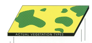
As the use of GIS became more common among natural resource management agencies and conservation organizations, there was interest in using habitat models to map species habitats and ranges, assess the hotspots of species richness, and design landscape strategies to protect biodiversity (Scott et al. 1993). This management strategy was not anticipated when agencies developed procedures to conduct habitat assessments, but it built on the fundamentals of habitat. Under the direction of the United States Geological Survey, a national program called the Gap Analysis Program (GAP) was initiated, which aimed to rapidly identify gaps in the protection of high biodiversity locations at a state level. First, the GAP program mapped vegetation types based on satellite data (Figure 7.3). Vegetation was considered a good integrator of physical and biological attributes because it includes attributes like elevation, soil types, climate, and slope. Then species-specific habitat models were developed that connect habitat types in the vegetation maps with other possible attributes in the GIS to map ranges of species. Many species of interest were mapped and locations of high biodiversity were identified. Then public lands, wildlife management areas, and parks were mapped to show gaps in the protection of biodiversity hotspots. This is the prominent comprehensive land conservation planning tool for biodiversity conservation.

USE OF CELLULAR AUTOMATA ANALYSIS
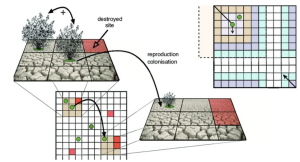
More recently, as larger scale environmental questions have come under analysis (e.g., whole ecosystems and landscapes), habitat modeling has been augmented to deal with larger spatial and temporal realms. Issues like change in climate, land use, and water regulation drove this endeavor to expand the way habitat is considered at much larger scales. The common approach adopted was cellular automata modeling around habitat conditions by cell (Itami 1994). Cellular automata modeling consists of a uniform grid of cells over an ecosystem or landscape, where thousands of cells can cover a study area (Figure 7.4). Each cell is connected to adjacent cells which exchange materials, like water and nutrients. Habitat models are embedded in each cell to predict the habitat status of each cell. The final result is a designation of a state or habitat type by cell, which can be used to generate a map of habitat variation across the ecosystem or landscape.
CELLULAR AUTOMATA EXAMPLES
Two landscape models were developed to predict habitat changes across a wetland-dominated landscape of south Louisiana due to the effects of water flow regulation across the Mississippi River Delta and climate change. These were the Coastal Ecological Landscape Spatial Simulation (Costanza et al. 1990) and the Barataria–Terrebonne Ecological Landscape Spatial Simulation (Reyes et al. 2000). Both study teams mapped changing habitat composition in 1 km2 cells for a portion of the delta strongly affected by controlled river flow. The cells were connected by flows of water, salt, nitrogen, sediments, and water elevation. The habitat model inside each cell included hydrodynamics, productivity, soil-dynamics, flooding, salinity, and other properties. Habitat switching was predicted using data input to the habitat models for each cell. The product resulted in a wetland landscape that could be determined under different river flow controls and climate change scenarios. The following habitat types were the results of the final classifications by cell: upland, freshwater marsh, swamp forest, brackish marsh, saline marsh, and open water. These habitat types were not defined by species requirements; rather, they were modeled using principles of habitat change. These analyses were done to cover multiple decades because the evolution of landscape properties takes many years under some scenarios. These landscape models were well developed and represent the expansion of habitat modeling in space and time.
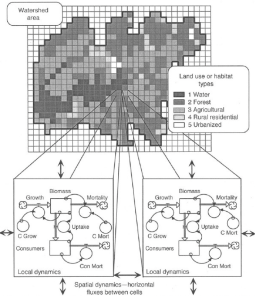
Expansion of habitat modeling was used to address ecosystem change in the Patuxent River basin in Maryland (Costanza et al. 2002) to evaluate future scenarios of development (Figure 7.5; Table 7.2). Regional socioeconomic trends were included to predict likely development pressures and outcomes. Consequences of different development patterns were explored by modeling flows, like nitrogen and phosphorus discharges into Chesapeake Bay. Other predicted outcomes were plant growth, runoff with dissolved nutrients, and formation of soils. Cells were classified by habitat type (water, forest, agriculture, residential, and urban), and adjacent cells could exchange water, nutrients, and suspended materials. Model runs inside each cell were elaborate. When the results were tallied across cells under each development scenario, one could predict for the landscape properties, map habitat types, and see the distribution of vegetation biomass and net primary production. Again, this extension of habitat modeling across large landscapes and far into the future was an advancement from researchers’ pioneering methods for larger scale habitat forecasting.
Table 7.2: Partial results of output from Patuxent landscape model used for decision-making. Source: Costanza et al. 2002

CASE STUDY: HABITAT ASSESSMENT IN THE FLORIDA EVERGLADES

In 1947, the Florida Everglades became the first national park designated to protect an ecological system (Figure 7.6). It has also been designated a United Nations Educational, Scientific and Cultural Organization (UNESCO) World Heritage Site, an International Biosphere Reserve, and a Wetland of International Importance (National Park Service 2021a). The restoration of the Everglades is a large ecosystem management case focused on habitat conservation issues. Its management program combines traditional habitat suitability indices with large scale hydrologic modeling to compare alternative water management policies. The traditional habitat suitability indices are just like those that the USFWS developed in the 1980s. These were combined with landscape level hydrologic simulation to portray what water management can achieve. The goal of the Everglades restoration program is on “getting the water right.” Over the past century, many canals were built for water drainage and about half of the Everglades has been lost to urban and agricultural conversion of land (Walker and Solecki 2004). Over time the Everglades has changed to an unhealthy ecosystem with more than 50 species on the United States Endangered Species Act list. Both Florida and the United States Congress passed Acts with the intent of restoring the Everglades to a more natural state at an estimated cost of several billion dollars. Their main focus was on quantity, quality, timing, and the distribution of water flow across this large landscape. This is a difficult and complex challenge because of the size of the ecosystem and its unique hydrology. In addition, there are many stakeholders involved who want to secure differing benefits from the Park. This is an informative case study, involving complicated ecology, hydrology, and human demands that uses fundamental habitat modeling in a new way.
The comparison of water management alternatives and planning options for the restoration of the Everglades engaged a diverse set of stakeholders, who were primarily interested in and concerned with choices. The comparison analysis needed to be easily understandable, transparent, and responsive to input. There were several models used to evaluate water management in the Everglades but they were complicated, specialized, and not easily modified (Fennema et al. 1994; DeAngelis et al. 1998). Non-specialists could not understand them, and often these models were called “black boxes.” The challenge was to get these diverse parties to engage with each other in the process of finding a solution for future management. This required all parties to have an understanding of the analyses and an ability to offer informative input. This Everglades case was shaped by its focus on habitat, which was easily understood and simulated across the landscape.
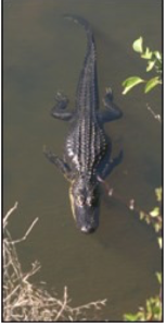
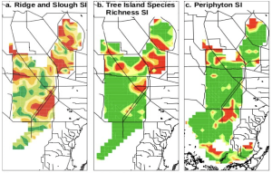
The analysis process began by identifying habitats that could be related to water depths, flows, and timing. The selected habitats were either key landscape features, support for groups of animals, or were in need of specific species. These habitats were important attributes of the Everglades Park from the public’s perspective The process identified five different habitats which characterized an ecosystem scale response to water management changes. Two landscape attributes were chosen to reflect changes in water management over decades: ridge and slough landscape habitats, and tree islands. Periphyton is a fast reacting indicator of water flows and quality, so it was included to act as an early warning signal if problems arose. One species group, fish in general, were identified to reflect conditions over time and space. These are notable biological features of the Everglades which readily respond to changes in the environment due to water management alterations. Finally, one species, the American alligator (Alligator mississippiensis), was identified for habitat assessment because of its ecological prominence and its recognition among the public (Figure 7.7).
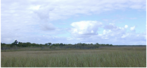
The ridge and slough landscape habitat is characteristic of the Everglades and is composed of sawgrass ridges and open waters (Figure 7.8). This complex habitat decreased in area during the canal building and drainage of the Everglades. Thus, it was selected as a habitat to be restored by water management, as it is considered a symbol of health for the Everglades. Tree islands are another component of the Everglades landscape (Figure 7.9). Tree islands serve as nesting sites for birds and reptiles, provide dry terrain for animals, and support more species than other habitat in the Everglades. Though a small portion (5-10%) of the Everglades landscape, they are critical for supporting wildlife. The periphyton habitat index was included as a sensitive indicator of hydrologic conditions and water quality, especially nutrients in a naturally oligotrophic system. Periphyton also has many effects on the ecosystem by influencing secondary production, nutrient concentrations, and dissolved gases. These three diverse habitats are indicative of the nature of the Everglades and characteristic of the landscape overall.
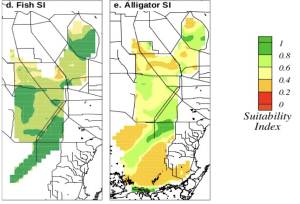
A modeling effort that combined the HSI approach and landscape simulation was developed (Tarboton et al. 2004). Fish and American alligators are both sensitive to habitat conditions. Fishes are important indicators of ecosystem status, and provide food for wading birds and alligators. When water is high, small fish flourish and become abundant, and occupy marshes where they are largely protected from predators in the vegetation. When the marshes dry, small fish are forced into confined watered areas where they are vulnerable to wading birds, alligators, and large fish. Fish abundance typically increases with time since the last marsh drying. This one multi-species group and the American alligator are interconnected, and are common images and biological features of the Everglades ecosystem.
The American alligator will be used to detail how habitat suitability indices are used for five habitats. Alligators are the top carnivore in the Everglades. They physically modify the ecosystem by developing water holes and trails. Water depths are important to alligators for different reasons: breeding, nest construction, nest flooding, and interaction between alligators. Four habitat factors were identified for alligators which were plotted against an influential hydrologic variable. The charts from habitat suitability indices and factors were plotted on a 0 to 1 scale, from non-habitat (0) to optimum habitat (1). This was a key decision point in the analysis process because it defined the fundamental data for comparison of water management alternatives and was used for evaluating ecosystem response. This study was done in English measurement units, so it is presented here using these same units.
For each of the five habitats, suitability indices were formed to link to hydrologic conditions (Figure 7.10). The number of days where the water was less than 0.5 feet deep influenced the proportion of adult female alligators expected to nest in a given year. This related to drought conditions that dispersed males and limited water habitats that caused physiological stress. Shorter periods of low water or marsh drying increased the suitability of the habitat for alligators. For nest construction, there was an optimal water depth during the period of mid-April to mid-May. After nests were constructed, it was important that water levels remain stable during the egg incubation period (mid-June to the end of August). Eggs were laid in the nest about 0.5 to 1.0 feet above water level, so if water levels rose more than 0.5 feet, some eggs would be flooded and not survive. During dry periods, alligators occupied water holes or other watered areas. They were crowded in these locations and small alligators were often eaten by large alligators. Therefore, alligator abundance went down because of limited water habitat in dry periods. Also, body condition decreased because of the lack of food. Optimal habitat conditions were marked by no loss of water level, as a water level reduction of 2 or 3 feet impacted alligator abundance and health. These four charts illustrate the conditions for water levels and the timing of changes (Figure 7.10). All five habitats had multiple charts like these, defining water management protocols for each primary habitat assessment feature.

For each of the five habitats, a consolidated index was made by doing a weighted arithmetic mean of the habitat suitability indices. The factors for the American alligator were weighted based on their expected impact on the overall population of alligators in the Everglades. The formula for alligators was:
Overall alligator suitability index =
(3 x SI breeding +
1 x SI survival and condition) / 9Where SI is the suitability index of each factor.
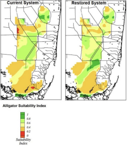
A simulation model was then required to produce a rendering of the hydrologic properties across the Everglades. Inputs values were the habitat suitability indices simulation of water depths, flow velocity, dry periods, and the period of water level change for a daily time step and for 2-mile by 2- mile grid cells spanning the region. Then each cell had a computed overall alligator suitability index (Figure 7.11). A map was made for each water management plan to see how it affected the five habitats (Figure 7.12).
Each of the five habitats were mapped using simulated outcomes of each water management plan. Interaction between interested individual stakeholders and organizations led to the selection of one management plan using the habitat quality maps (Loucks 2006). Other analyses were performed, but the main result was that the restoration water management plan was selected. The analysis process was easy to understand and engaged everyone with an interest in the matter. Participants over their differences which enabled them to agree upon the selection of a single restoration plan. Again, this exercise entailed applying habitat suitability indices to a complex landscape problem which linked water management, physical conditions, and ecological restoration together within a unique and expansive ecosystem.
SUMMARY
Habitat assessment is used for a variety of purposes like animal stocking levels, planning restorations, determining the need for habitat rehabilitation, comparing future development scenarios, and assigning mitigation actions for habitat losses. Advancements in the science of habitat assessment and new habitat modeling options in GIS have led to better prediction of the distribution of species and design of conservation programs. These new advancements help to address many of the core issues at the heart of habitat assessment and provide the basis for stakeholder engagement and cooperation in developing solutions to changing situations on the ground.
REFERENCES
Anderson, R.P., Lew, D. and Peterson, A.T., 2003. Evaluating predictive models of species’ distributions: criteria for selecting optimal models. Ecological modelling, 162(3), pp.211-232.
Ashley, P. and Muse, A., 2008. Habitat Evaluation Procedures Report; Graves Property-Yakama Nation (No. P106586). Bonneville Power Administration (BPA), Portland, OR.
Bain, M.B. and Stevenson, N.J., 1999. Aquatic habitat assessment. Asian Fisheries Society, Bethesda.
Beutel, T.S., Beeton, R.J.S. and Baxter, G.S., 1999. Building better wildlife habitat models. Ecography, 22(2), pp.219-219.
Brooks, R.P., 1997. Improving habitat suitability index models. Wildlife Society Bulletin, 25, pp.163- 167.
Costanza, R., Sklar, F.H. and White, M.L., 1990. Modeling coastal landscape dynamics. BioScience, 40(2), pp.91-107.
Costanza, R., Voinov, A., Boumans, R., Maxwell, T., Villa, F., Wainger, L. and Voinov, H., 2002. Integrated ecological economic modeling of the Patuxent River watershed, Maryland. Ecological monographs, 72(2), pp.203-231.
DeAngelis, D.L., Gross, L.J., Huston, M.A., Wolff, W.F., Fleming, D.M., Comiskey, E.J. and Sylvester, S.M., 1998. Landscape modeling for Everglades ecosystem restoration. Ecosystems, 1(1), pp.64-75.
Dussault, C., Courtois, R. and Ouellet, J.P., 2006. A habitat suitability index model to assess moose habitat selection at multiple spatial scales. Canadian Journal of Forest Research, 36(5), pp.1097-1107.
Elton, C., 1927. Animal ecology, 1927. Sidgwick & Jackson, LTD, London, 56.
Fennema, R.J., Neidrauer, C.J., Johnson, R.A., MacVicar, T.K. and Perkins, W.A., 1994. A computer model to simulate natural Everglades hydrology. Everglades: The ecosystem and its restoration, pp.249-289.
Fielding, A.H. and Bell, J.F., 1997. A review of methods for the assessment of prediction errors in conservation presence/absence models. Environmental conservation, 24(1), pp.38-49.
Franklin, J., 2010. Mapping species distributions: Spatial inference and prediction. Cambridge University Press. New York, NY.
Fraser, D.F. and Sise, T.E., 1980. Observations on stream minnows in a patchy environment: a test of a theory of habitat distribution. Ecology, 61(4), pp.790-797.
Fretwell, S.D., and Lucas, H.L., 1970. On territorial behavior and other factors influencing habitat distribution in birds. I. Theoretical development. Acta Biotheoretica, 19, pp.16-36.
Fretwell, S.D., 1972. Populations in a seasonal environment. Princeton University Press, Princeton, NJ.
Grinnell, J., 1917. The niche-relationships of the California Thrasher. The Auk, 34(4), pp.427-433.
Guisan, A. and Zimmermann, N.E., 2000. Predictive habitat distribution models in ecology. Ecological modelling, 135(2-3), pp.147-186.
Guisan, A. and Thuiller, W., 2005. Predicting species distribution: offering more than simple habitat models. Ecology letters, 8(9), pp.993-1009.
Gurnell, J., Clark, M.J., Lurz, P.W., Shirley, M.D. and Rushton, S.P., 2002. Conserving red squirrels (Sciurus vulgaris): Mapping and forecasting habitat suitability using a Geographic Information Systems Approach. Biological conservation, 105(1), pp.53-64.
Gustafson, E.J., 1998. Quantifying landscape spatial pattern: What is the state of the art? Ecosystems, 1(2), pp.143-156.
Hall, L.S., Krausman, P.R. and Morrison, M.L., 1997. The habitat concept and a plea for standard terminology. Wildlife society bulletin, pp.173-182.
Hirzel, A.H., Le Lay, G., Helfer, V., Randin, C. and Guisan, A., 2006. Evaluating the ability of habitat suitability models to predict species presences. Ecological modelling, 199(2), pp.142-152.
Hirzel, A.H. and Le Lay, G., 2008. Habitat suitability modelling and niche theory. Journal of applied ecology, 45(5), pp.1372-1381.
Hutchinson, G.E., 1957. Cold spring harbor symposium on quantitative biology. Concluding remarks, 22, pp.415-427.
Itami, R.M., 1994. Simulating spatial dynamics: Cellular automata theory. Landscape and urban planning, 30(1-2), pp.27-47.
Knight, T.W. and Morris, D.W., 1996. How many habitats do landscapes contain? Ecology, 77(6), pp.1756-1764.
Loucks, D.P., 2006. Modeling and managing the interactions between hydrology, ecology and economics. Journal of Hydrology, 328(3-4), pp.408-416.
Meixler, M.S., 2021. A species-specific fish passage model based on hydraulic conditions and water temperature. Ecological Informatics, p.101407.
Meixler, M.S., Bain, M.B. and Walter, M.T., 2009. Predicting barrier passage and habitat suitability for migratory fish species. Ecological Modelling, 220(20), pp.2782-2791.
Milhous, R.T., Wegner, D.L. and Waddle, T., 1984. User’s guide to the physical habitat simulation system (PHABSIM) (No. 11). Department of the Interior, United States Fish and Wildlife Service. Washington, DC.
Mitra, S. and Bezbaruah, A.N., 2014. Railroad impacts on wetland habitat: GIS and modeling approach. Journal of Transport and Land Use, 7(1), pp.15-28.
National Park Service, 2021a. Florida: Everglades National Park. Available: https://www.nps.gov/articles/everglades.htm (September 2021).
National Park Service, 2021b. American alligator: Species profile. Available: https://www.nps.gov/ ever/learn/nature/alligator.htm (September 2021).
Pianka, E.R., 1966. Latitudinal gradients in species diversity: A review of concepts. The American Naturalist, 100(910), pp.33-46.
Pulliam, H.R., 2000. On the relationship between niche and distribution. Ecology letters, 3(4), pp.349- 361.
Reyes, E., White, M.L., Martin, J.F., Kemp, G.P., Day, J.W. and Aravamuthan, V., 2000. Landscape modeling of coastal habitat change in the Mississippi Delta. Ecology, 81(8), pp.2331-2349.
Rosenzweig, M.L., 1981. A theory of habitat selection. Ecology, 62(2), pp.327-335.
Rushton, S.P., Ormerod, S.J. and Kerby, G., 2004. New paradigms for modelling species distributions? Journal of applied ecology, 41(2), pp.193-200.
Sardanyés, J., Piñero, J. and Solé, R., 2019. Habitat loss‐induced tipping points in metapopulations with facilitation. Population Ecology, 61(4), pp.436-449.
Schamberger, M. and Krohn, W.B., 1982. Status of the habitat evaluation procedures. United States Fish and Wildlife Service publications 48. Washington, DC.
Schamberger, M. and O’Neil, J., 1986. Concepts and constraints of habitat model testing. Pages 5-10 in J. Verner et al., eds. Wildlife 2000. University of Wisconsin Press, Madison, WI.
Scott, J.M., Davis, F., Csuti, B., Noss, R., Butterfield, B., Groves, C., Anderson, H., Caicco, S., D’Erchia, F., Edwards Jr, T.C. and Ulliman, J., 1993. Gap analysis: A geographic approach to protection of biological diversity. Wildlife monographs, pp.3-41.
Southwood, T.R., 1977. Habitat, the templet for ecological strategies? Journal of animal ecology, 46(2), pp.337-365.
Stalnaker, C., Lamb, B. L., Henriksen, J. , Bovee, K., and Batholow, J., 1995. The instream flow incremental methodology: A primer for IFIM. U. S. Department of the Interior, Biological Report 29, Fort Collins, CO.
Tarboton, K.C., Irizarry-Ortiz, M.M., Loucks, D.P., Davis, S.M. and Obeysekera, J.T., 2004. Habitat suitability indices for evaluating water management alternatives. Office of Modeling Technical Report, South Florida Water Management District, West Palm Beach, FL.
Theuerkauf, S.J. and Lipcius, R.N., 2016. Quantitative validation of a habitat suitability index for oyster restoration. Frontiers in Marine Science, 3, p.64.
Turner, M.G., O’Neill, R.V., Gardner, R.H. and Milne, B.T., 1989. Effects of changing spatial scale on the analysis of landscape pattern. Landscape ecology, 3(3), pp.153-162.
United States Fish and Wildlife Service, 1980a. Habitat as a basis for environmental assessment. Ecological Services Manual 101. Division of Ecological Services, United States Fish and Wildlife Service, Department of the Interior, Washington, DC.
United States Fish and Wildlife Service, 1980b. Habitat Evaluation Procedures (HEP), Ecological Services Manual 102. Division of Ecological Services, United States Fish and Wildlife Service, Department of the Interior, Washington, DC.
United States Fish and Wildlife Service, 1981. Standards for the development of habitat suitability index models. Ecological Services Manual 103, United States Fish and Wildlife Service, Washington, DC.
United States Geological Survey, 2021a. Habitat suitability map and change between 2011 and 2014. Available: https://www.usgs.gov/media/images/habitat-suitability-map-and-change-between-2011-and- 2014 (September 2021).
United States Geological Survey, 2021b. Tree islands. Available: https://www.usgs.gov/media/images/ tree-islands (September 2021).
Urich, D.L. and Graham, J.P., 1983. Applying habitat evaluation procedures (HEP) to wildlife area planning in Missouri. Wildlife Society Bulletin (1973-2006), 11(3), pp.215-222.
Walker, R. and Solecki, W., 2004. Theorizing land-cover and land-use change: The case of the Florida Everglades and its degradation. Annals of the Association of American geographers, 94(2), pp.311-328.
Zajac, Z., Stith, B., Bowling, A.C., Langtimm, C.A. and Swain, E.D., 2015. Evaluation of habitat suitability index models by global sensitivity and uncertainty analyses: A case study for submerged aquatic vegetation. Ecology and evolution, 5(13), pp.2503-2517.
Zorn, T.G., Seelbach, P.W. and Wiley, M.J., 2011. Developing user-friendly habitat suitability tools from regional stream fish survey data. North American Journal of Fisheries Management, 31(1), pp.41- 55.

